Tanker Drift

On 3 March, the LNG tanker MT Arctic Metagaz was struck by suspected Ukranian naval drones. The vessel has been adrift since then, and in a testament to South Korean maritime engineering remaining afloat after an LNG explosion (with the front decidedly not falling off).

The complete lack of any visualization of where the drifting tanker was and where it might go was bothering me. So here’s my go at it, with the caveat that I am using only public info and limited understanding.

Opendrift, (which you can read about more in my sea slime post) has a Ship Drift module, so I thought why not use that! The length and beam I got from marine traffic, and I used Claude to come up with an estimate for height and draft

o.seed_elements(lon=13.5667, lat=35.3000, radius=250, number=1000,
                time=start_time,
                length=277, beam=43.0, height=28.0, draft=11.5)

The initial seed position I got from this post by the Department of fisheries.

Opendrift uses current, wave and wind information to act on, in this case, 1000 seeded particles and model their trajectory.

Surface currents were downloaded from the Copernicus Marine Service Mediterranean Sea Physics Analysis and Forecast product, specifically the dataset cmems_mod_med_phy-cur_anfc_4.2km-2D_PT1H-m. This provides hourly, two-dimensional surface current fields (eastward and northward velocity) at approximately 4.2 km horizontal resolution.

Wave-induced Stokes drift was obtained from the companion Mediterranean Sea Waves Analysis and Forecast product dataset cmems_mod_med_wav_anfc_4.2km_PT1H-i, which provides hourly wave parameters at the same 4.2 km resolution using the WAM Cycle 6 wave model forced by ECMWF atmospheric fields.

Wind at 10 metres above sea level was streamed in real time from the NCEP Global Forecast System (GFS) via the Pacific Islands Ocean Observing System (PacIOOS) THREDDS Data Server, providing global 0.25-degree resolution atmospheric model output covering the simulation period.

I ran the simulation in a python notebook and saved it to netcdf.

As for the actual plotting:

# Malta Shape
malta_sf <- gisco_get_countries(country = "MLT", resolution = "01") 

ggplot() +
  geom_sf(data = malta_sf) +
  geom_path(data = df, aes(lon, lat, group = particle, color = date),
            alpha = 0.2, linewidth = 0.6, lineend = "round",
            linejoin = "round") +
  geom_point(data = df %>% group_by(particle) %>% slice(1),
             aes(lon, lat), color = "red", size = 1) +
  scale_color_viridis_c(
    option = "plasma",
    breaks = as.numeric(seq(
      as.POSIXct("2026-03-12", tz = "UTC"),
      as.POSIXct("2026-03-19", tz = "UTC"),
      by = "1 day"
    )),
    labels = function(x) format(as.POSIXct(x, origin = "1970-01-01", tz = "UTC"), "%b %d")
  ) +
  labs(
    title = "ARCTIC METAGAZ — Drift Simulation",
    subtitle = "1000 points Starting at: 35°18′N, 13°34′E — March 14 2026, 4pm",
    color = "Date",
    x = NULL, y = NULL
  ) +
  theme_minimal(base_size = 12) +
  theme(
    plot.title    = element_text(face = "bold"),
    panel.grid    = element_line(color = "grey92"),
    legend.position = "right"
  )+
  geom_sf()+
  coord_sf(ylim = c(34.5, NA))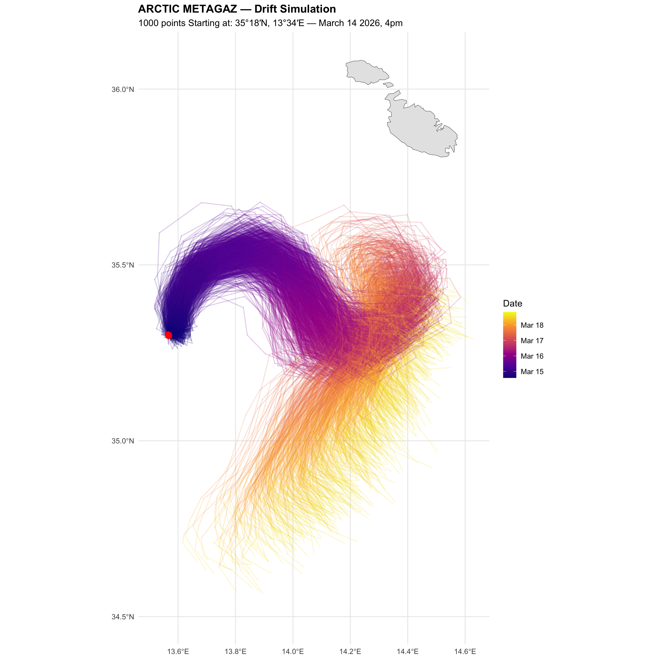

The ship will meander quite a bit, since the wind is forecast to keep changing over the coming days.

Since we seeded 1000 particles, we can think of it as a Monte Carlo simulation (each particle gets a slightly different starting position, and OpenDrift adds random perturbations to each one’s trajectory at every time step.)