Introduction
I suppose a defining feature of being in your mid twenties is that you find progressively more of your small talk having to do with properties: how big they should be, which floor negates the value added by a lift, and even, when alternate conversation seems especially hard to conjure, the benefits of using one type of grout as opposed to another.
Often during such conversations, I found myself wondering how much value can be extracted by an in-depth analysis. So when I came across a local property website that seemed relatively straightforward to scrape, I decided to make a weekend project of it!
The Dataset
I’d estimate that around half my time on this was spent trying to extract meaningful variables, but in the end, I managed to end up with just shy of 1,500 listed properties. The two main continuous variables in this dataset are the price of the property listing in Euros, and the size in square meters. The number of bedrooms and bathrooms was also harvested, together with a whole set of categorical variables including Town, Region, the floor where applicable, and whether a property was listed as having a Garage/Views/Pool/Lift/Garden/Airconditioning/an Outside Area/if it’s Furnished.
Now, I’d advise against using this data to make inferences about current property prices, since this is what people are asking for their property. This particular website might not even be representative of the market, because for example it might be more popular in one region of the island as opposed to another.
str(PropertyListingsCleaned)## spec_tbl_df [1,394 x 19] (S3: spec_tbl_df/tbl_df/tbl/data.frame)
## $ Listing Name : chr [1:1394] "Malta property: Townhouse in Zabbar for sale" "Property Malta: Spacious 3 Bedroom Apartment in Balzan" "Gozo Real Estate: 5 Bedroom House in Gharb for sale" "Property for sale in Malta: Furnished 2 Bedroom Apartment in St. Julians" ...
## $ PropertyID : chr [1:1394] "Prop4" "Prop5" "Prop6" "Prop7" ...
## $ Bedrooms : chr [1:1394] "2" "3" "5" "2" ...
## $ Bathrooms : chr [1:1394] "2" "2" "6" "2" ...
## $ Furnished : chr [1:1394] "No" "No" "No" "Yes" ...
## $ Views : chr [1:1394] "No" "No" "Yes" "Yes" ...
## $ Garage : chr [1:1394] "No" "No" "No" "No" ...
## $ Pool : chr [1:1394] "No" "No" "Yes" "No" ...
## $ Outside : chr [1:1394] "Yes" "Yes" "Yes" "Yes" ...
## $ Floor : chr [1:1394] NA "1st" NA "4th" ...
## $ Lifts : chr [1:1394] "No" "Yes" "No" "Yes" ...
## $ Airconditioning: chr [1:1394] "No" "No" "No" "No" ...
## $ Garden : chr [1:1394] "No" "No" "Yes" "No" ...
## $ TextDescription: chr [1:1394] "Location: Zabbar Malta property for sale is this Townhouse in Zabbar for sale. Although the property needs some"| __truncated__ "Location: Balzan Property in Malta for sale is this spacious 3 bedroom apartment located in Balzan in a small b"| __truncated__ "Location: Gozo - Gharb Agents from our Gozo Real Estate agency are presenting this beautiful shell form house i"| __truncated__ "Location: St. Julians Furnished 2 Bedroom Apartment in St. Julians with sea vies is brought toy ou from our lis"| __truncated__ ...
## $ PriceEuros : num [1:1394] 160000 308000 424000 630000 365000 365000 425000 175000 285000 275000 ...
## $ AreaMSquared : num [1:1394] 108 147 600 100 109 137 110 90 120 120 ...
## $ Town : chr [1:1394] "Zabbar" "Balzan" "Gharb" "St. Julians" ...
## $ Region : chr [1:1394] "Southern Harbour" "Western" "Gozo" "Northern Harbour" ...
## $ PropertyType : chr [1:1394] "Townhouse" "Apartment" "House" "Apartment" ...
## - attr(*, "spec")=
## .. cols(
## .. `Listing Name` = col_character(),
## .. PropertyID = col_character(),
## .. Bedrooms = col_character(),
## .. Bathrooms = col_character(),
## .. Furnished = col_character(),
## .. Views = col_character(),
## .. Garage = col_character(),
## .. Pool = col_character(),
## .. Outside = col_character(),
## .. Floor = col_character(),
## .. Lifts = col_character(),
## .. Airconditioning = col_character(),
## .. Garden = col_character(),
## .. TextDescription = col_character(),
## .. PriceEuros = col_double(),
## .. AreaMSquared = col_double(),
## .. Town = col_character(),
## .. Region = col_character(),
## .. PropertyType = col_character()
## .. )Exploring the data
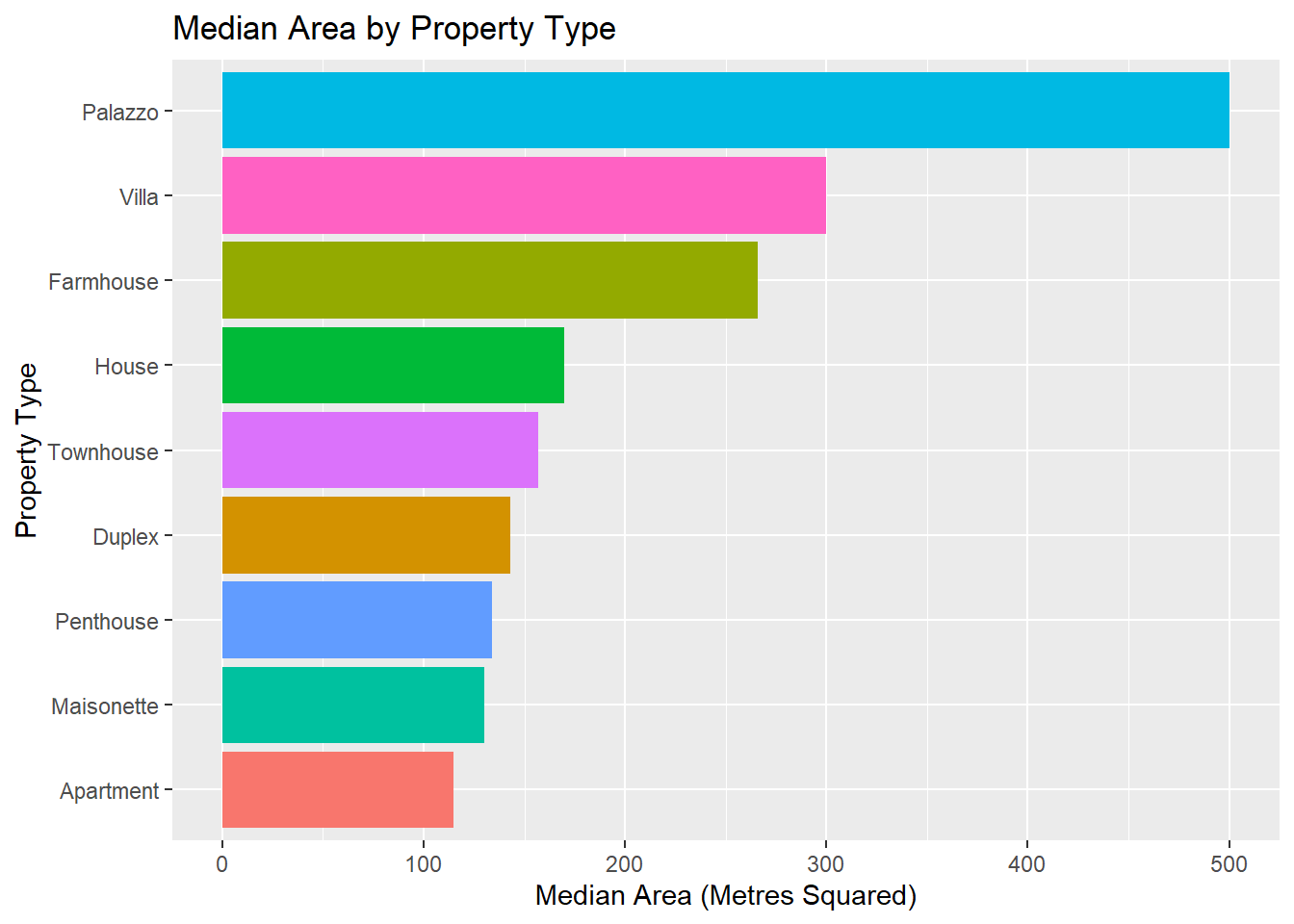
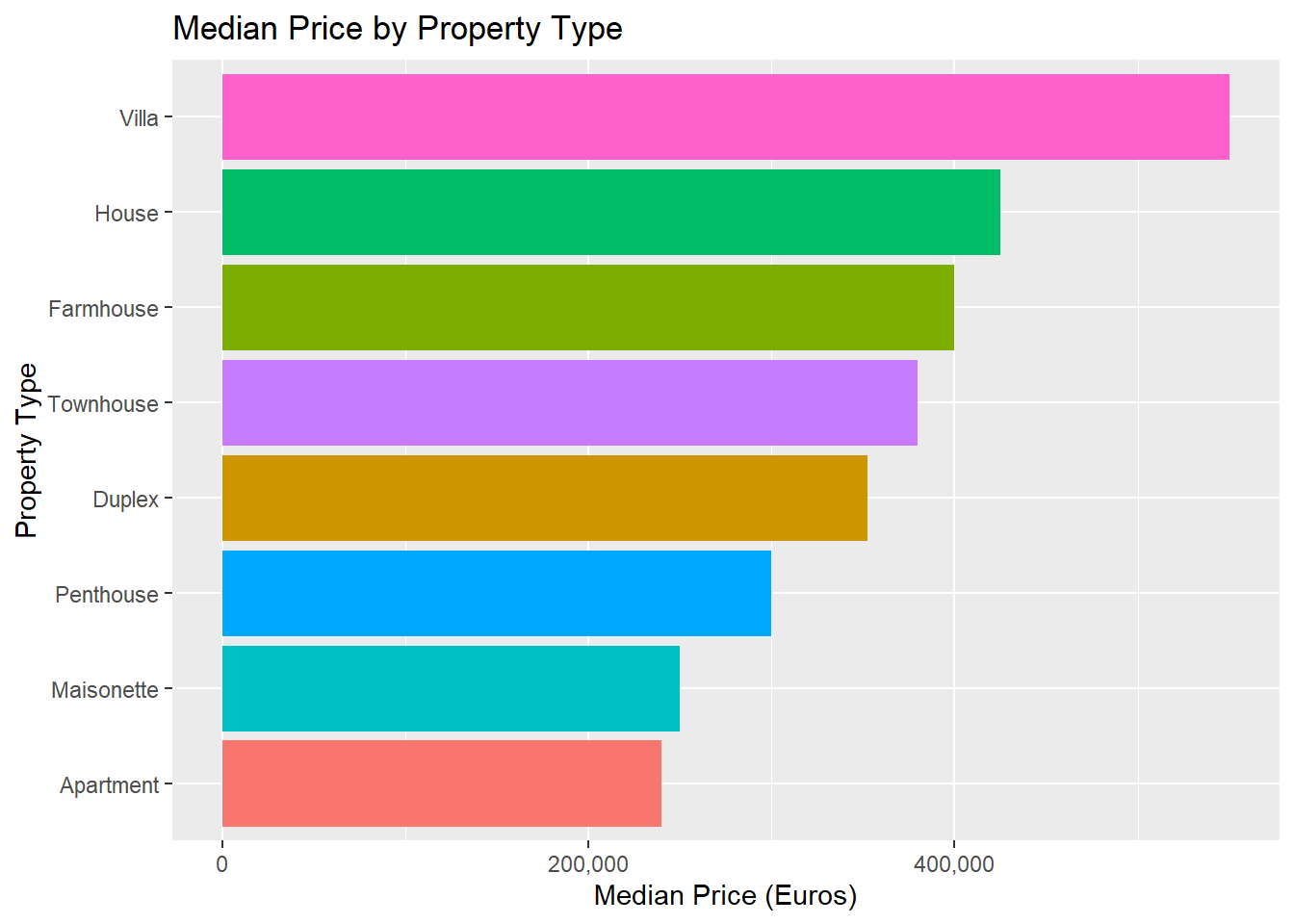
It turns out that the median listed price of a property on this particular website is 280,000 Euros, and the median area is 131 square meters. Here’s how price is distributed, split by property type:
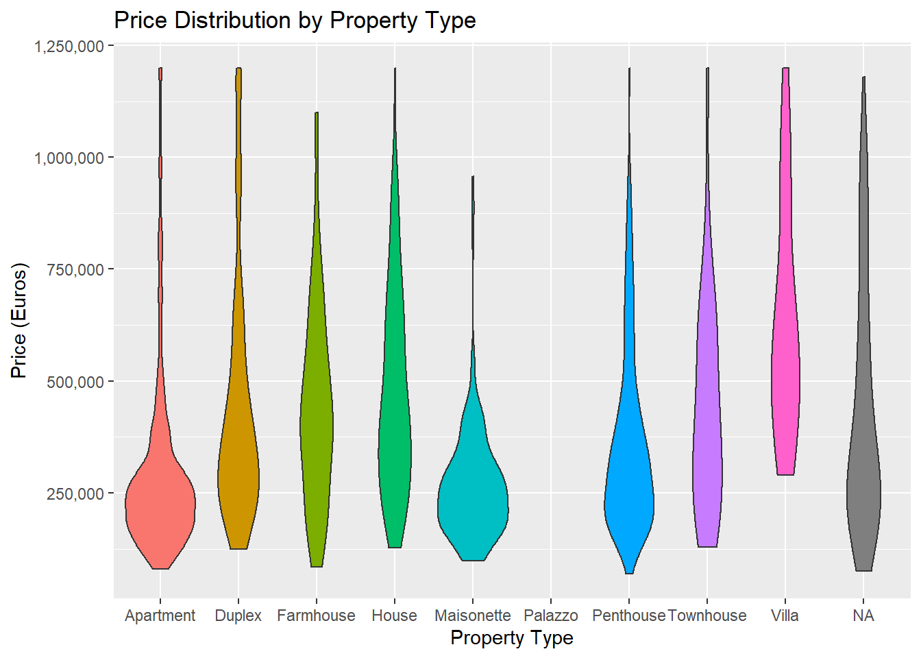
You can see that most apartments and maisonettes have an asking price of around 250,000 Euros, while duplexes, farmhouses and houses tend to be more variable. And a villa might cost you anywhere from 250,000 Euros to 2.5 Million.
How does Cost vary with Area?
When you initially plot cost and area, the graph looks wholly uninformative, since prices and areas tend to have a few large values that hinder us from seeing any meaningful pattern.
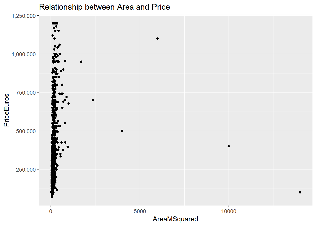
To fix this, we’ll use a log 10 transformation that just rescales the data.
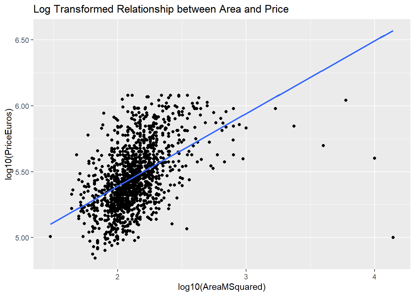
And there you have it! intuitevly, the price of a property has a linear relationship with it’s area!
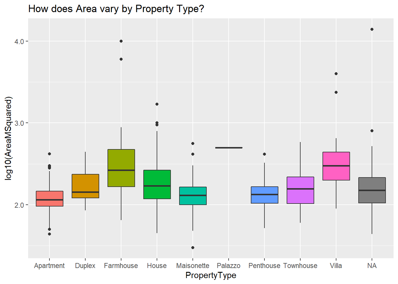
Since this is a log10 transformation, to get the area in meters squared back, just multiply 10 by the power of that number. So, for instance, eyeballing the above, our apartments have a median area of 2.1. 10^2.1 is 125, which makes sense.
##More exploration:
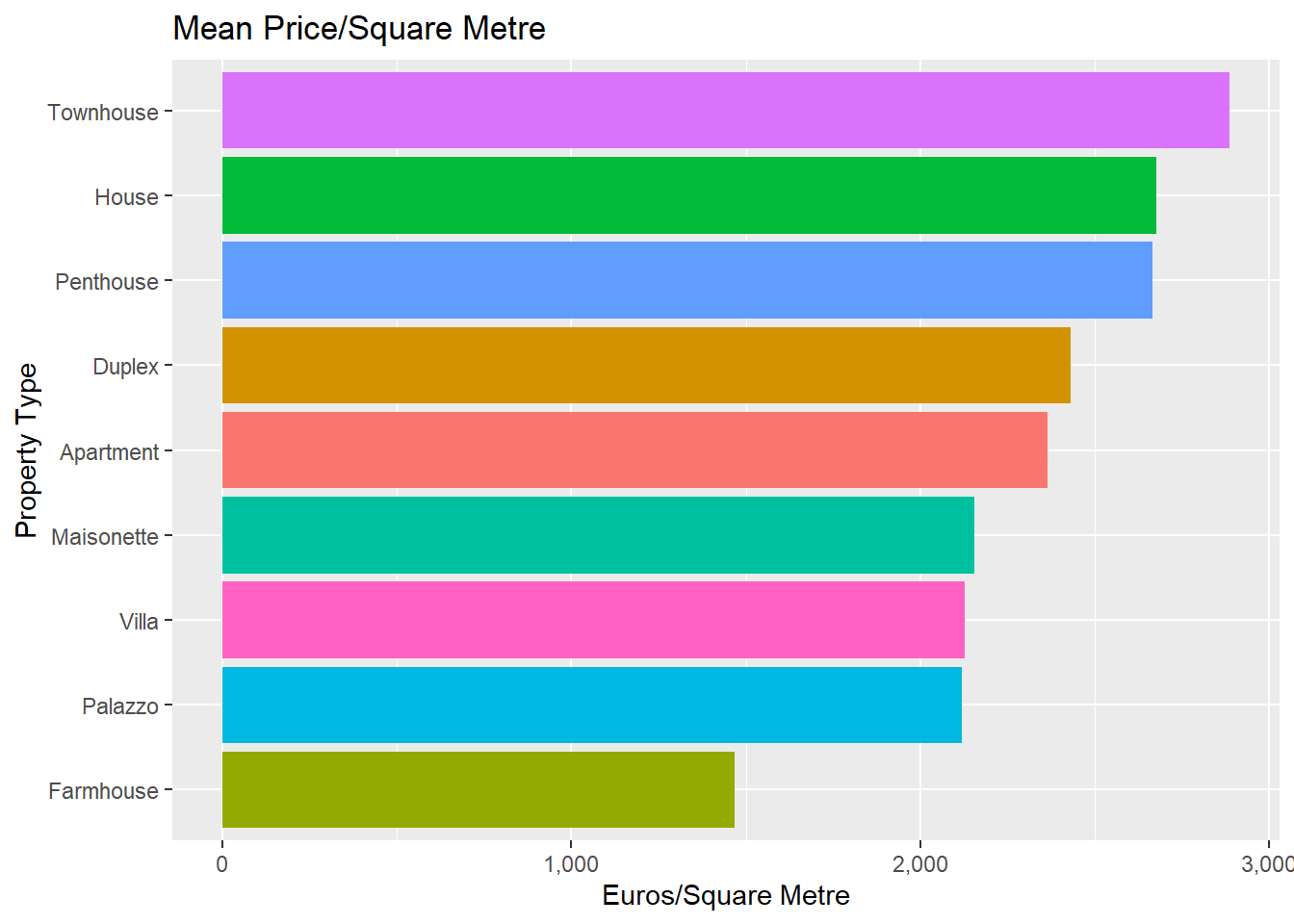
What’s the cost of a metre square?
This is an interesting one. What’s the actual cost of a metre square by property type?
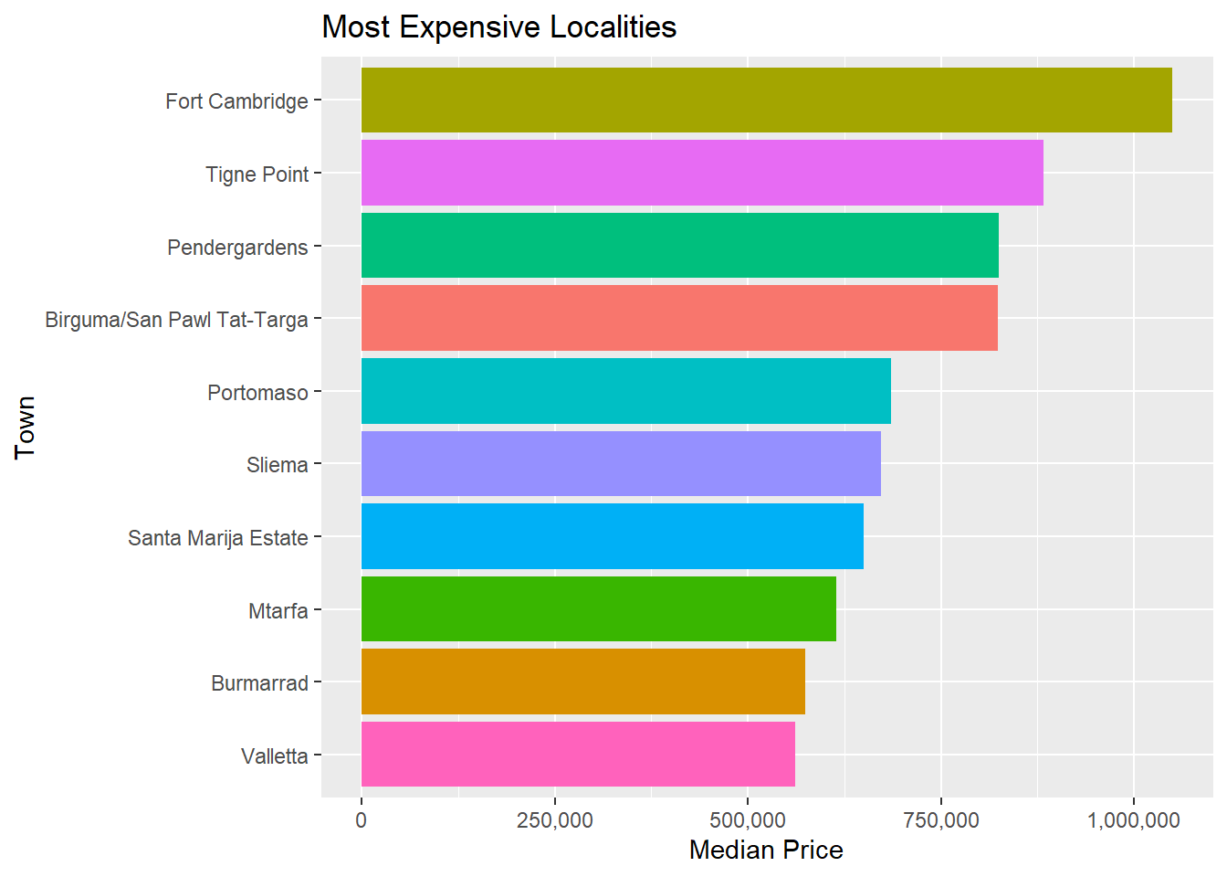
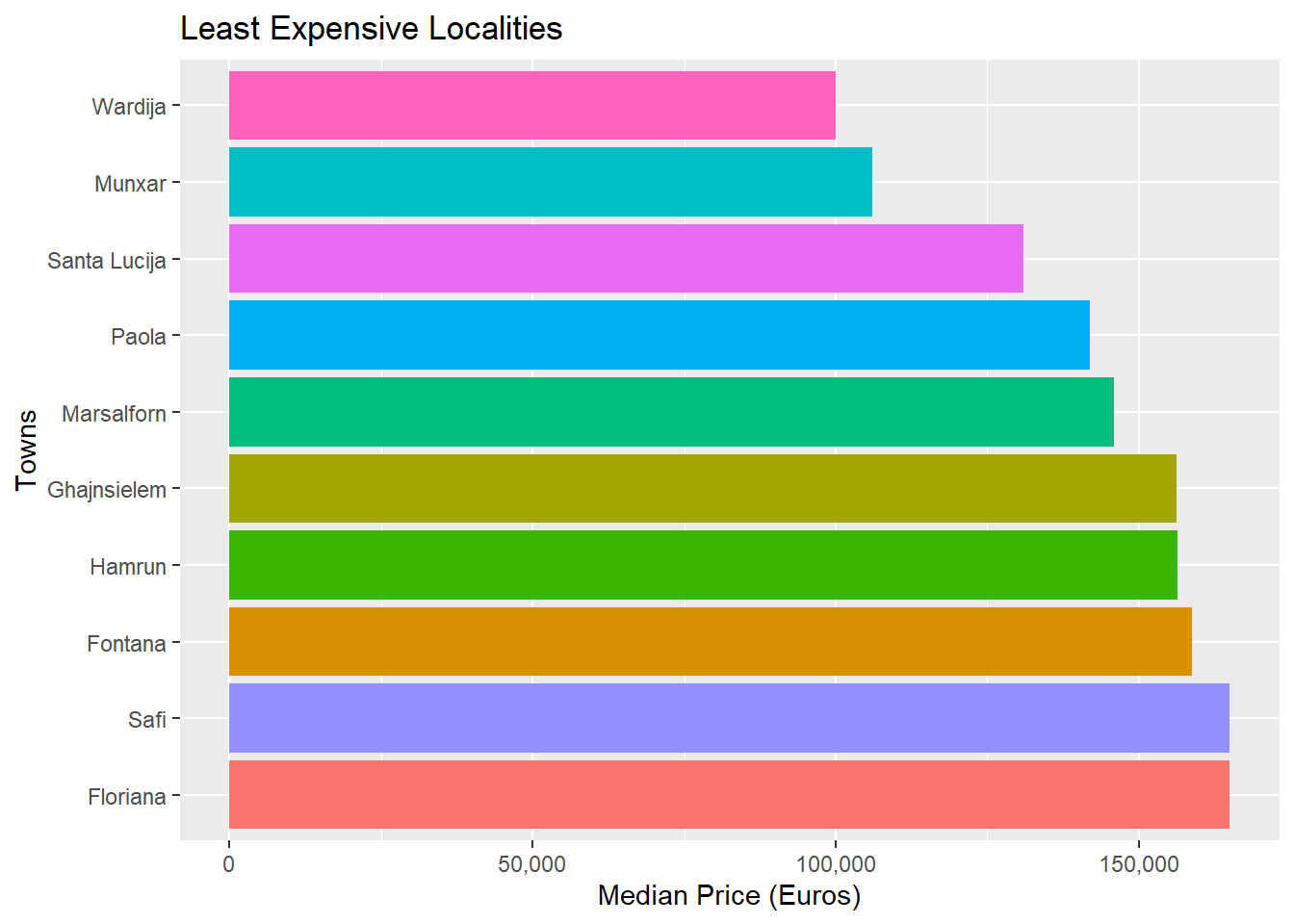
##Are there differences based on locality?
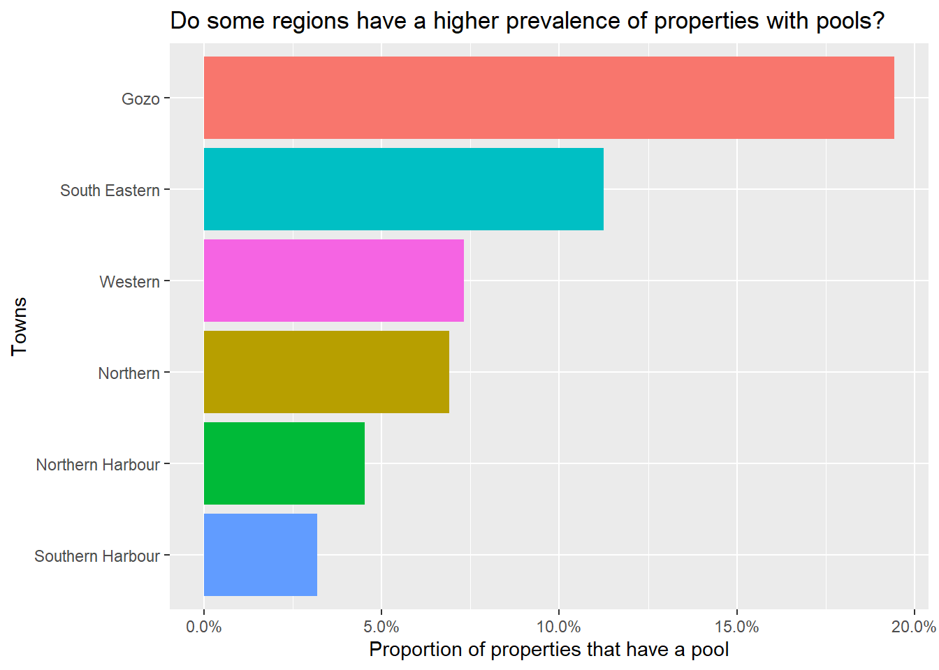
It looks like pools are more common in rural regions like Gozo and the South East, and become less common as we move into the much more heavily urbanised North and South Harbour regions.
Pondering the nice things
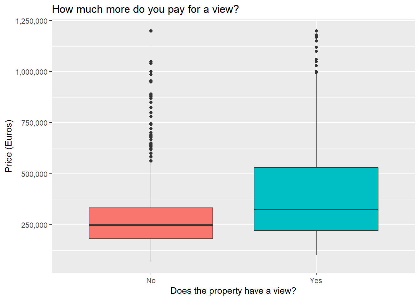
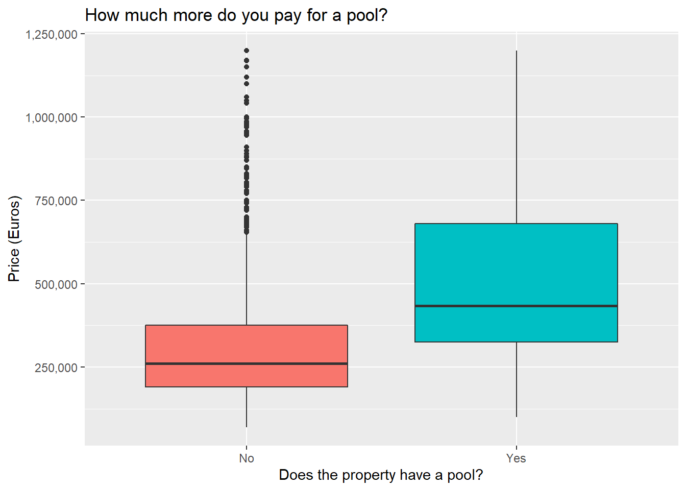
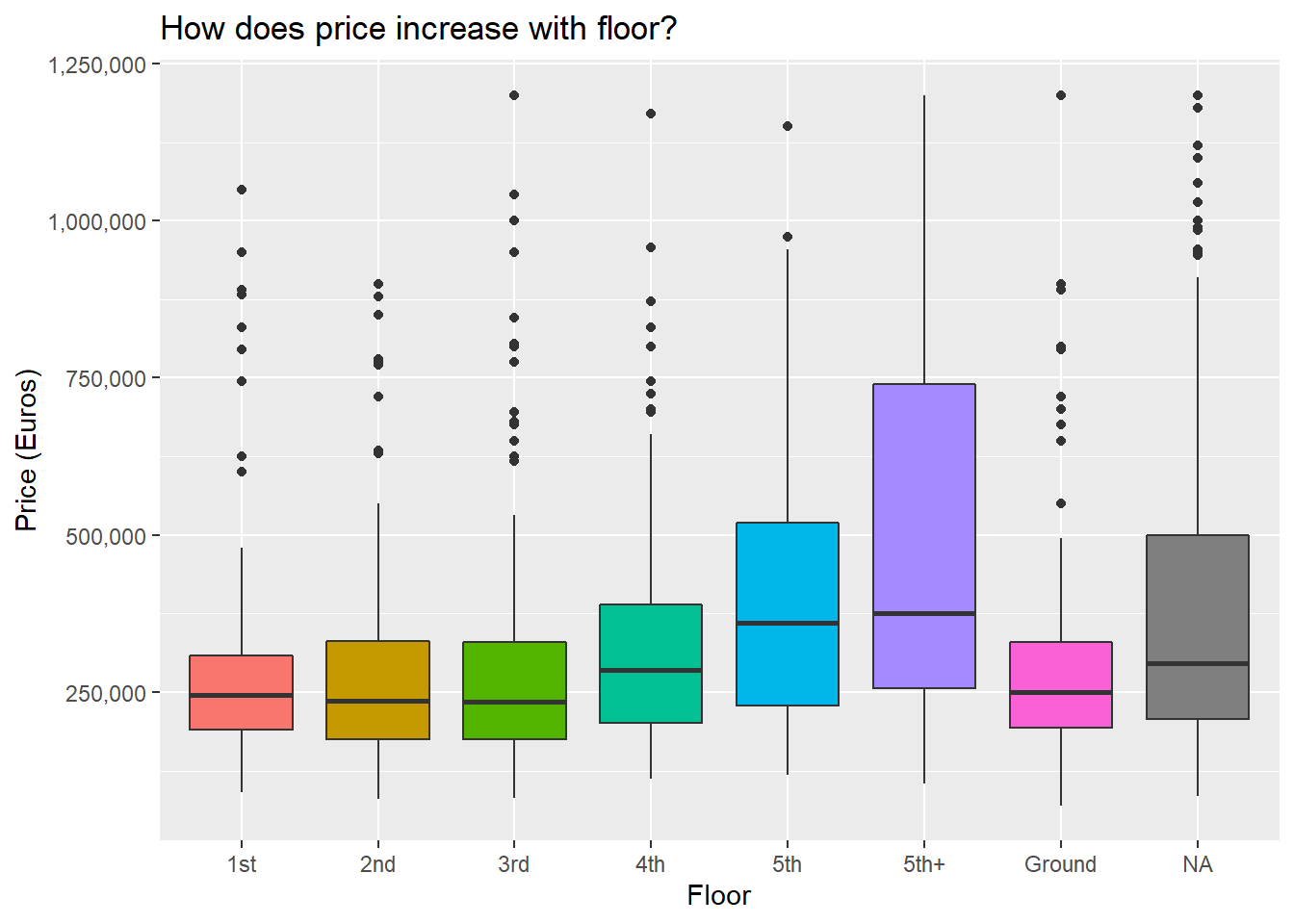
Seems pretty intuitive so far. Having a pool or a view and being higher up all lead to higher prices. That being said, it’s not ideal to look at these variables in isolation like this, since for instance having a pool might also be associated with a higher prevalence of having a view or having a larger property area. To which will you then attribute the increase in property price?
The correct way would be to deploy a linear model!
##Linear Modeling Time!
First, let’s fit a linear model to the relationship between price and area of a property.
CompleteCases <- PropertyData[complete.cases(PropertyData), ]
SimpleLM <- lm(PriceEuros ~ AreaMSquared, data = CompleteCases)
summary(SimpleLM)
##
## Call:
## lm(formula = PriceEuros ~ AreaMSquared, data = CompleteCases)
##
## Residuals:
## Min 1Q Median 3Q Max
## -1329012 -104891 -51301 37925 894860
##
## Coefficients:
## Estimate Std. Error t value Pr(>|t|)
## (Intercept) 212789.62 10450.99 20.36 <2e-16 ***
## AreaMSquared 769.59 60.61 12.70 <2e-16 ***
## ---
## Signif. codes: 0 '***' 0.001 '**' 0.01 '*' 0.05 '.' 0.1 ' ' 1
##
## Residual standard error: 187500 on 959 degrees of freedom
## Multiple R-squared: 0.1439, Adjusted R-squared: 0.143
## F-statistic: 161.2 on 1 and 959 DF, p-value: < 2.2e-16Our bare bones linear model tells us that the average price of a listed property is 212,789 euros, and goes up by 769 euros each additional square metre we add. However the R-squared value, which tells us how well our model fits the data is dreadful, showing we manage to explain only around 14% of the variance in the data.
What happens if we throw in every single variable we have?
ComplexLM <- lm(PriceEuros ~ ., data = CompleteCases)
summary(ComplexLM)
##
## Call:
## lm(formula = PriceEuros ~ ., data = CompleteCases)
##
## Residuals:
## Min 1Q Median 3Q Max
## -878308 -81683 -19755 57216 868419
##
## Coefficients:
## Estimate Std. Error t value Pr(>|t|)
## (Intercept) -146604.33 32379.79 -4.528 6.74e-06 ***
## Bedrooms 70314.67 7874.32 8.930 < 2e-16 ***
## FurnishedYes 56521.62 14996.56 3.769 0.000174 ***
## ViewsYes 107325.53 12411.47 8.647 < 2e-16 ***
## GarageYes<U+00A0> 60619.90 18031.16 3.362 0.000805 ***
## PoolYes 80551.43 24619.57 3.272 0.001108 **
## OutsideYes -6267.82 16687.28 -0.376 0.707296
## Floor2nd 2050.15 18653.18 0.110 0.912505
## Floor3rd 7798.87 18628.55 0.419 0.675567
## Floor4th 1057.65 19885.07 0.053 0.957594
## Floor5th 36664.60 25285.27 1.450 0.147384
## Floor5th+ 114338.63 21881.82 5.225 2.15e-07 ***
## FloorGround -4371.11 20395.97 -0.214 0.830350
## LiftsYes 18291.82 17962.25 1.018 0.308777
## GardenYes -473.76 45164.39 -0.010 0.991633
## AreaMSquared 312.86 65.46 4.779 2.04e-06 ***
## RegionNorthern 160001.74 15083.39 10.608 < 2e-16 ***
## RegionNorthern Harbour 217959.53 14495.74 15.036 < 2e-16 ***
## RegionSouth Eastern 79074.55 22542.78 3.508 0.000473 ***
## RegionSouthern Harbour 129294.90 23123.59 5.591 2.96e-08 ***
## RegionWestern 175645.85 21773.26 8.067 2.20e-15 ***
## PropertyTypeDuplex 41084.88 30743.88 1.336 0.181758
## PropertyTypeFarmhouse 263123.62 90679.83 2.902 0.003799 **
## PropertyTypeHouse 165116.48 40890.20 4.038 5.83e-05 ***
## PropertyTypeMaisonette 28404.07 21819.88 1.302 0.193323
## PropertyTypePenthouse 5339.11 16021.79 0.333 0.739028
## PropertyTypeTownhouse 142456.80 60452.77 2.356 0.018654 *
## PropertyTypeVilla 90696.54 98381.15 0.922 0.356825
## ---
## Signif. codes: 0 '***' 0.001 '**' 0.01 '*' 0.05 '.' 0.1 ' ' 1
##
## Residual standard error: 147800 on 933 degrees of freedom
## Multiple R-squared: 0.4829, Adjusted R-squared: 0.468
## F-statistic: 32.27 on 27 and 933 DF, p-value: < 2.2e-16We’re now managing to explain 46% of the variance present in the dataset, as well as being able to assess the relative importance of the features.
For instance, if a property is furnished, the addition to the value is around 56,500 euros. If this seems high, it might be because other factors are at play. For instance, a large number of properties listed as unfurnished might be in shell status, requiring further work, resulting in them being listed at a lower price.
Floor was an interesting one: the only statistically significant effect was when a property was higher than the 5th floor. For the priviledge of looking down on 4 floors, you’ll fork out an extra 114,338 euros.
Price also goes up by 70,000 Euros for each additional bedroom(this is probably measuring the same thing as area, since these two measures are probably highly correlated), and the steepest premiums are paid to live in the Northen Harbour (~217k Euros) and Western (~175k Euros) regions respectively.
I think we can do better.
Onwards to Decision Trees!
In my experience it’s pretty hard explaining the above to a general audience, and the linear model framework was not fitting overly well. So let’s try another framework that might be better at this, with the added bonus that it’s easier to understand.
Decision trees split the data into sub populations using the variables it thinks generate the best splits. To test the quality of the decision tree we’ll be building, I’ve split the data randomly. We’ll use 80% of it to train our model, and 20% of it to assess it’s performance on new “unseen” data.
##Generate Train/Test Split
set.seed(2019)
sample <- sample.int(n = nrow(CompleteCases), size = floor(.8*nrow(CompleteCases)), replace = F)

train <- CompleteCases[sample, ]
test  <- CompleteCases[-sample, ]
The benefits of decision trees are twofold: they might pick up on complex non-linear relationships that linear modeling can’t, and they produce wonderful intuitive graphs like this one:
library(rpart)
library(rpart.plot)

tree <- rpart(PriceEuros ~ ., data = train, cp = 0.02)

rpart.plot(tree, box.palette="RdBu",)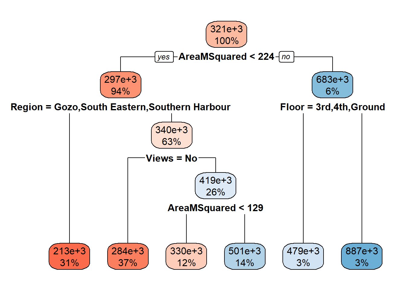
What our decision tree is telling us, starting from the top, is that it thinks that the average price of a property is 322,000 Euros. Then comes the first split: the model has determined that the best variable to split on is area. If the area is less than 213 metres squared, we go left. 93% of the listed properties fall under this bracket.
It’s also decided to split one more time using area. If our property’s area is less than 129 metres squared, we go left once again. Region now becomes important. If we’re in Gozo, we go left again. 12% of our properties meet this criteria, and their price is around 164,000 Euros. For the 41% of properties with an area less than 129 metres squared that are not in Gozo, their price is around 265,000 euros. This tells us that property in Gozo is cheaper.
Let’s go back up to area is less than 129 metres squared and go right this time. Here we’re saying no, so our property is larger than 129 metres squared, but smaller than the 213 of the split above it. Let’s pretend our region isn’t Gozo, South Eastern or Southern Harbour, so right once again. Now whether our property has a view becomes a factor. This is where it might get a bit counterintuitive. If Views = No is yes, that is, the property does not have a view, its listed price is around 344,000 Euros. If a property has a view, it’s listed price jumps up to 516,000 Euros - these are probably your Portomaso apartments and Siggiewi villa’s.
So how good is our single humble tree at predicting?
TreePreds <- predict(tree, test)

library(Metrics)# Has a handy inbuilt RMSE function!
rmse(TreePreds, test$PriceEuros)
## [1] 179939.9Not overly good: on average it’s off by 146,000 euros.
Just to give you an idea of what that looks like in real life, here are the first 5 predictions of the model using the test data that it’s never seen before, compared with the actual price these properties were listed at:
data.frame("PredictedPrice" = TreePreds, "ActualListedPrice" = test$PriceEuros) %>%
  head()
## PredictedPrice ActualListedPrice
## 1 283533.2 308000
## 2 283533.2 285000
## 3 500771.6 295000
## 4 283533.2 260000
## 5 283533.2 200000
## 6 283533.2 274000It’s pretty close on the 1st, 2nd and 6th occasion, but way off on the 3rd, 4th and 5th. Part of the reason might be that these are listed requested prices, and some sellers are more optimistic than others. Take the 2nd and 3rd case for instance. The model predicted the same value, which probably means it saw similar regional/area/view etc. splits in both cases.
We can easily confirm this if we look at the 2nd and 3rd rows of our testing data:
test[2:3,]## # A tibble: 2 x 13
## Bedrooms Furnished Views Garage Pool Outside Floor Lifts Garden PriceEuros
## <dbl> <fct> <fct> <chr> <fct> <fct> <chr> <fct> <fct> <dbl>
## 1 3 Yes No No No Yes 2nd No No 285000
## 2 1 No Yes No No Yes 4th Yes No 295000
## # ... with 3 more variables: AreaMSquared <dbl>, Region <fct>,
## # PropertyType <fct>And indeed, the only difference is in bedrooms and region, but the listed price varies dramatically. Let’s beef up our approach: instead of one tree, we’ll grow many, and average their outputs. To do this we’ll use the Caret package.
library(caret)## Loading required package: lattice##
## Attaching package: 'caret'## The following objects are masked from 'package:Metrics':
##
## precision, recall## The following object is masked from 'package:purrr':
##
## liftmyControl <- trainControl(method = "cv", number = 5, verboseIter = TRUE)
model_rf <- train(PriceEuros ~ .,
data = train,
tuneLength = 1,
method = "rf",
trControl = myControl,
importance = T)## + Fold1: mtry=5
## - Fold1: mtry=5
## + Fold2: mtry=5
## - Fold2: mtry=5
## + Fold3: mtry=5
## - Fold3: mtry=5
## + Fold4: mtry=5
## - Fold4: mtry=5
## + Fold5: mtry=5
## - Fold5: mtry=5
## Aggregating results
## Fitting final model on full training setplot(model_rf$finalModel)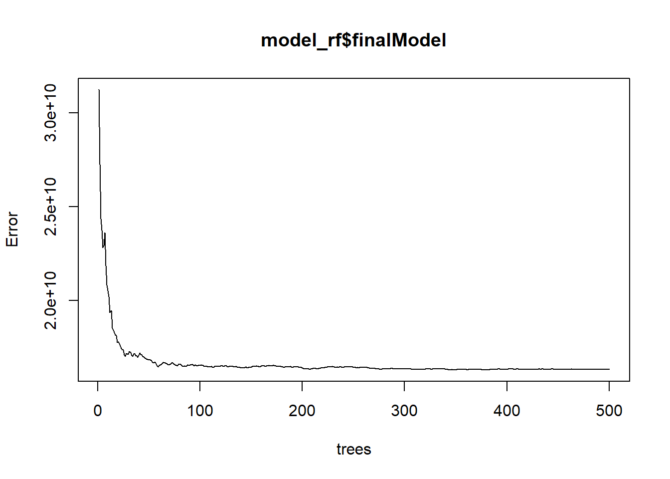
The above is the random forest in action, reducing the error as it fits progressively more decision trees. There are marginal accuracy returns beyond 50 trees, and by 100 the plateau tells us that each additional tree is not worth the computation time.
So, did this procedure increase accuracy? Let’s find out!
rfpred <- predict(model_rf, test)
rmse(rfpred, test$PriceEuros)
## [1] 155831data.frame("PredictedPrice" = rfpred, "ActualListedPrice" = test$PriceEuros) %>%
head()## PredictedPrice ActualListedPrice
## 1 275093.7 308000
## 2 251821.0 285000
## 3 341402.5 295000
## 4 227519.7 260000
## 5 208858.2 200000
## 6 236022.4 274000Yes! We’ve reduced our error to 128,000 euros! At this point, if the end aim of this excersise was to train a model to predict the price of a listing based on attributes, we’d probably go back to the data and try to scale and create more meaningful variables.
But it’s not, and since this post is getting long as it is, I’ll show you one last advantage of random forests: we can also use them to see which features it thinks are important! Which was sort of the point of all of this!
varImp(model_rf)$importance %>%
  as.data.frame() %>%
  rownames_to_column() %>%
  arrange(Overall) %>%
  mutate(Feature = forcats::fct_inorder(rowname)) %>%
  ggplot(aes(x=Feature, y=Overall)) +
  geom_point(col="tomato2", size=3) +
  geom_segment(aes(x=Feature,
                   xend=Feature,
                   y=min(Overall),
                   yend=max(Overall)),
               linetype="dashed",
               size=0.1) +
  labs(title="Overall Importance of Feature",
       subtitle = "As Assessed by Random Forest")+
       ylab("Importance") +
  coord_flip()+
  theme_classic()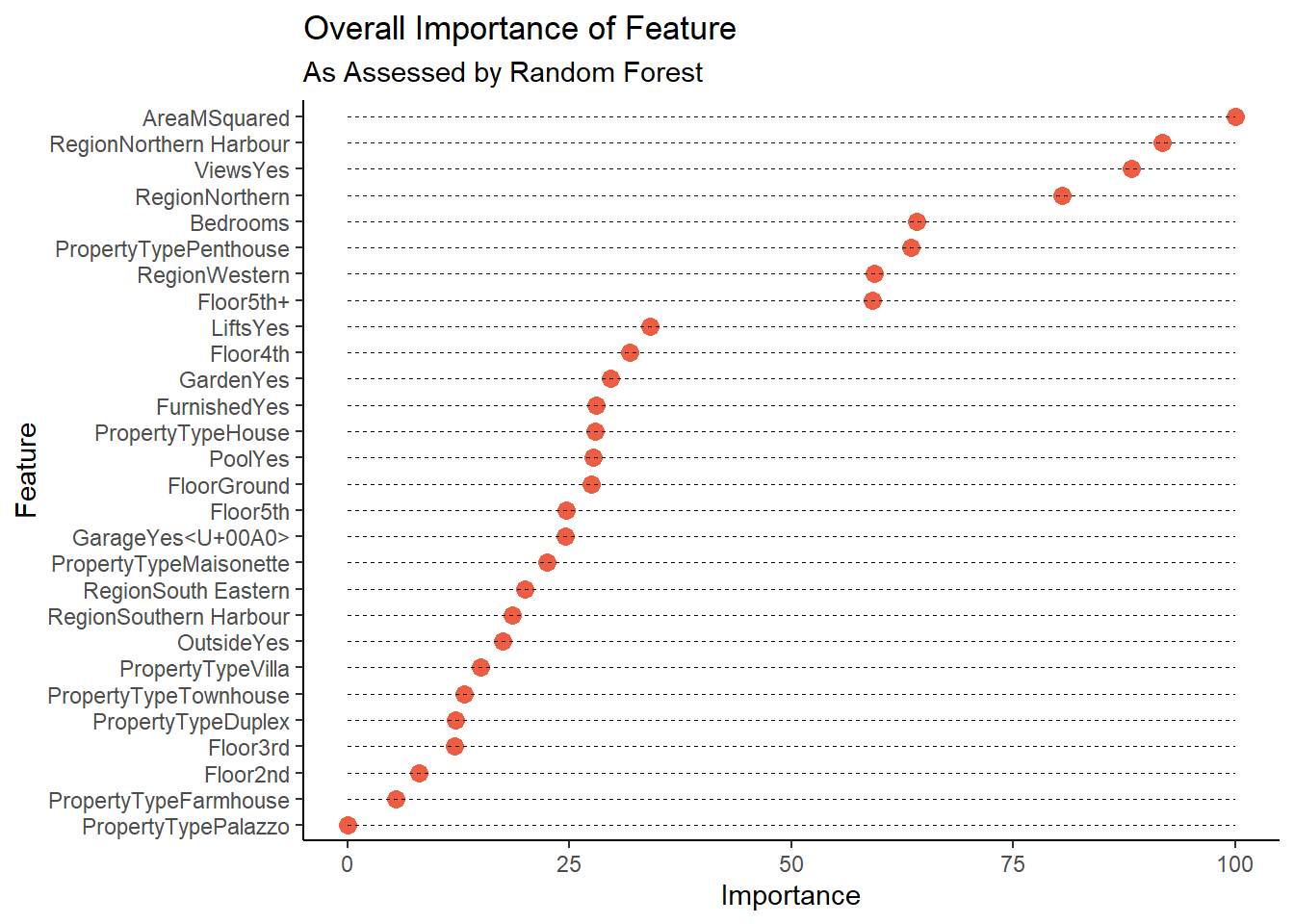
Perhaps the best way to think about the above would be as a ranking of which features generate the cleanest, most pure splits. These might not necessarily be the ones that add most value to a property, but they help us distinguish between a less expensive and a more expensive listing.