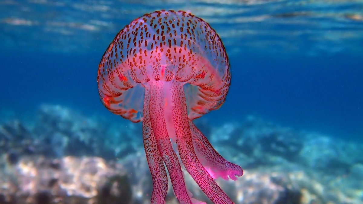
For nearly three years I’ve been obsessing over a side quest to build a jellyfish forecast for Malta. I’ve wanted to do this partly because it aligns with the stuff I like (machine learning + geospatial stats + maps) and partly to get myself down to the beach more in summer.
There’s also a neat little vibe I get from maps with predictions on static websites like this. I guess they hark back to the days when the internet was less ads/more information and I wanted my corner of this too.
The TL;DR of this post is that I did not succeed: the generated forecasts are too unreliable to be disseminated in any meaningful form. Instead, what this post will be is:
- a public sourcing of the labels I’ve gathered for this project in the hope someone smarter than me can crack it.
- a broad overview of the different approaches I tried. For posterity.
In many ways it does feel strange writing a post about a project that did not pan out, but I believe there is merit to failing in public and writing out these ‘what did not work’ posts. I will also aspire to give the introduction I wish I had when I started on this task 3 years ago.
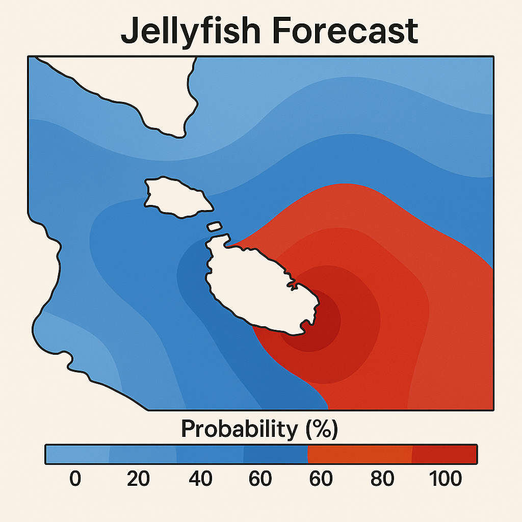
Yes, I got so excited about this at a point I even mocked up what the final product would look like ¯\_(ツ)_/¯
Just Give Me the Labels and Shut up
I ended up getting labels for two places, Malta and Spain.
Malta
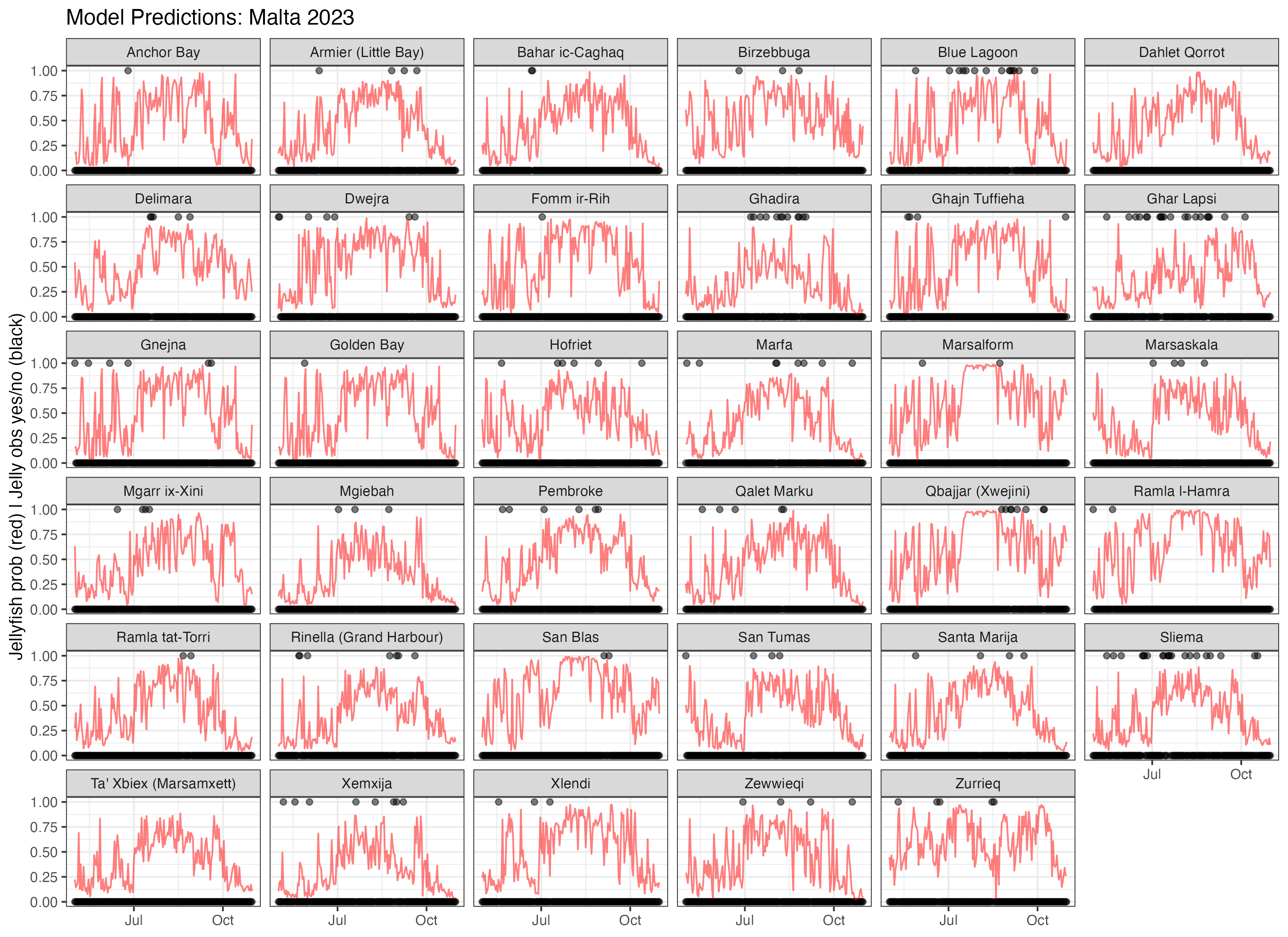
jelly_observations_all.csv is essentially just a scrape of the spot the jellyfish campaign’s website. There are two variations of the presence label, jelly or just pelagia_noctiluca. There are also a very small number of labeled absences.
malta_beach_locations.csv is a useful supplement on beach locations. orient is what direction the beach faces (I got this very manually from Google maps.)
Spain
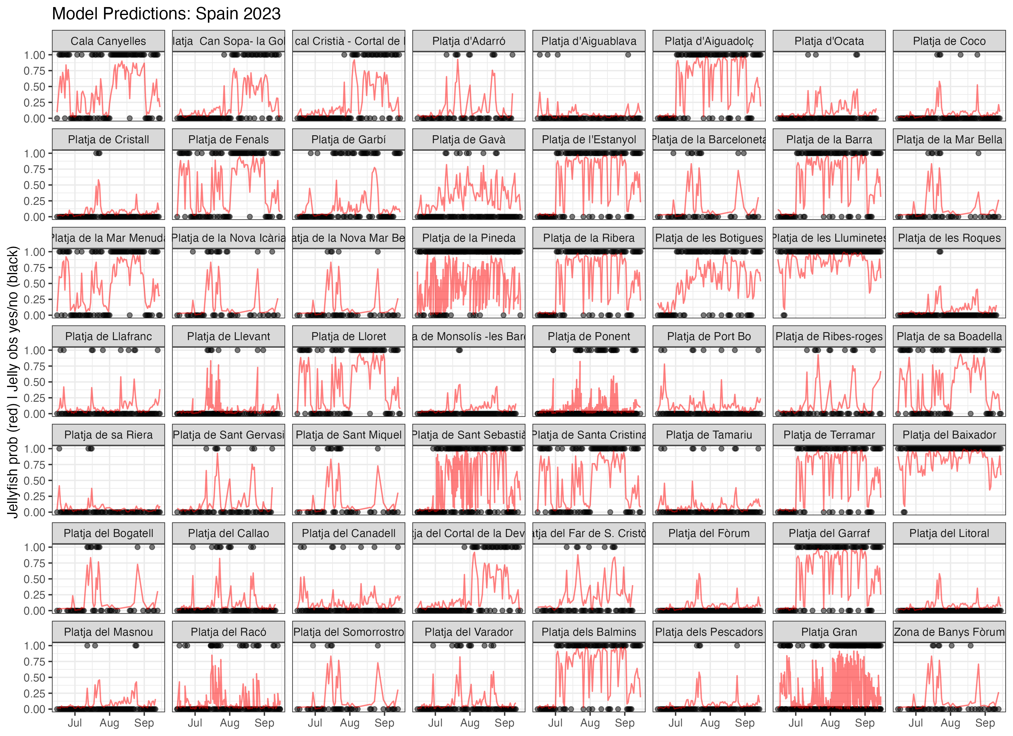
With such a vast coastline and a huge tourism industry, Spain’s jellyfish monitoring and research programs are probably the Mediterranean’s best funded, especially in Catalonia. The Catalonian Water Agency operates this interactive website with beach information, including jellyfish advisories which I scraped for the duration of 2023 and 2024 here.
Why Jellyfish are Hard to Predict
The most immediately noticeable hardship is a lack of public occurrence data. The only public data from academic research is a monthly overview from this paper. But to operationalise this into a valuable forecast, daily occurrences are the minimum granularity required, which means I had to get hacky and scrape my own.
In reality, that is only where the problems start. Since most of the labels are provided by the public, there are implicit biases, like for instance to report presence of jellyfish but not absence. It’s very hard to train models with data like this because the no label can mean either ‘no jellyfish’ or ‘no person to see a jellyfish’.
It’s also very easy to open yourself up to confounders in this set up. For instance, most of the jellyfish present labels are in summer. A very naive model would probably link jellyfish occurrence to temperature. Except, summer is when most people head to the beach and are prone to report sightings.
There’s an even more subtle version of this. Sandy beaches have more observations than rocky ones. Is rocky vs. sandy an important distinction for jellyfish… or is it that many more people frequent sandy beaches? But wait, the confound can be nested even deeper. These citizen science programs always experience a surge when they’re demoed in a school, since children naturally get pretty excited about this stuff and want to report. How many parents you know take their children to rocky beaches?
Then comes another whammy. The problem tends to be massively class imbalanced, that is, relatively speaking, there are much few days with jellyfish at a particular location. This makes sense: if they were present all the time we wouldn’t need a forecast. But this also means we need additional massaging for a model not to just learn to predict ‘no jellyfish’ all the time and be right most of the time.
Lastly, there is the humble jellyfish itself: I don’t think nature has created another being quite as nonplussed as this. Jellyfish will happily tolerate an exceptional range of conditions that would drive other species away. This means that covariates like salinity or sea temperature, which ordinarily might be useful for more sensitive species, lose predictive power. And while they might be still useful indirectly (for estimating predation via sea turtles for instance), this also means we have to adopt a time series approach or at the very least lag these features.
Surely this has Been Done Before
The only mature product I could find was JellyX, but it appears to have been taken off the market as of now. From what I saw the general idea is also employed in large scale commercial fishing to estimate the best fishing grounds at a particular time (instead of jellyfish you’d be predicting your commercial species of interest).
I should add, there are commercial interests for jellyfish forecasts too: Pelagia noctiluca blooms have shut whole beaches in Spain, interrupted with fish farming and shut down power plants when they clogged the cooling water supply.
General Approach
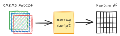
I got the majority of features from Copernicus Marine Service (CMEMS), and a very general Python script heavily using xarray would find the nearest cell to a beach point, interpolate when missing (the CMEMS land mask would sometimes obscure some points) and save to a table format.
The most involved feature engineering I did was work out a headwind component for each beach using the [uo, vo] components for wind and current. And in no particular order, some of the covariates I tried were (usually to around 300m of depth where available):
currents
wind
salinity
temperature
mixed layer thickness
sea surface height
chlorophyll a mass
phytoplankton mass
nutrients (nh4/no3/po4)
nppv
o2
I did also experiment with more annual measures to try to capture bloom dynamics (like temperature/rain/El Niño anomalies).
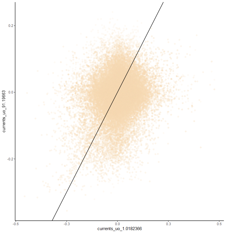
And in case you are like me an oceanography noob and wondering, yes there is a considerable amount of variation with depth. Here’s how much the uo component varies in about 90 m of water:
and here’s plankton mass: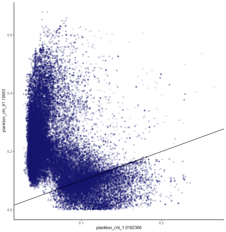
If you had to ask me why I leaned on CMEMS so heavily, my answer would be that it is the best dataset I know of that goes back far enough and that I could count on easy updates in the future if it panned out. Although I will add another painpoint was merging the reanalysis (pre 2023 data) to the forecast (post 2023 data) products. Another reason is that in my most optimistic and naive stages I also thought it would be easy to expand from Malta to the rest of the Mediterranean once I cracked it for here.
That being said parts of CMEMS are probably “too large” for this task as well. As an example, I was never completely satisfied with the realism of currents in the Gozo Channel, and since then I’ve learned actual oceanographers use CMEMS as an input to more local specialised models. I’m not sure this would have of made the meaningful difference though.
Models tried:
XGBoost/LightGBM
My first stop were gradient boosted tree models (I mostly settled on LightGBM). Here each date/beach location was a row, and the main way of encoding time was through feature lags (typically 3 or 7 days).
Besides the massaging via class weights to handle the imbalance, I also played around with a Tweedie loss function for these models (which in theory should have of handled the zero inflated data better).
I tried to make these types of models work for a long time because I had already gotten the ‘how to ship this’ part sorted in my mind (via daily github action), and the relatively simple ‘flat table’ input would have of made this easy.
I should also note that the most robust way of handling the class imbalance was to just show the model more positive classes. I did this in a variety of ways, in the end, undersampling the majority class worked about as well as generating synthetic minority class data – and the model trained faster (without even touching on the cost of synthetic data generation).
Speciality Zero Inflated
I also went down the speciality zero inflated model rabbit hole more thoroughly, following blog posts like Andrew Heiss’s one here.
In general, the idea is cool, but these models took forever to run, I had to be much more selective about features and didn’t improve the bottom line.
Maxent
It also turns out that ecologists have been struggling with the presence only label problem for a while and have developed their own elegant models for just this problem. In practice Maxent gave sensible predictions and solved the class imbalance problems. It, with the final iterations of the tree based models topped out at around an AUC of 0.66-0.68.
But Maxent also has it’s quirks: its a bit slow to run, quite sensitive to initial configuration and most packages like dismo in R depend on installing a Java virtual machine: the thought of doing this via github actions was already giving me nightmares. In the end, there weren’t any worthy gains that offset the additional complexity.
One other cool thing about MaxEnt I should mention is that many of the packages have been optimised to take in NetCDF as an input without the intermediate generating a table step.
Agent Based Framework
There’s this really cool paper by Joe El Rahi which treats this as an agent based model and doesn’t use machine learning at all. Essentially it builds on the opendrift framework and creates a custom Pelagia noctiluca agent that grows in 4 stages. In each of these stages El Rahi set up the jellyfish to swim at different speeds (Pelagia noctiluca can control it’s vertical position within the water column, swimming up after sunset and down after sunrise, but it is at the mercy of currents for horizontal movement).
The whole model is then spawning a large number of jellyfish, having them swim up and down the water column at different speeds as they grow and track where they end up when you input currents.
I did get this to work but I had very little correlation between beachings in the model and my observed jellyfish occurrences. Also there were a few small annoying quirks, like the tendency for my jellyfish to drift out of the area, beach at Sicily en masse, or get stuck going around the same gyre for months on end.
Neural Networks
I tried to take advantage of some of the time series info by creating sequences of n preceding days for each label for a Temporal Convolutional Networks. The n days in practice was a hyperparameter: I tried from 1 to 30 days, but I settled on 14 days in the end since it seemed to be a nice compromise. Besides having to pull all the old tricks from the tree based models to handle the class imbalance they tended to over-fit on the training data and loss would plateau very early.
Constant Factor Modification
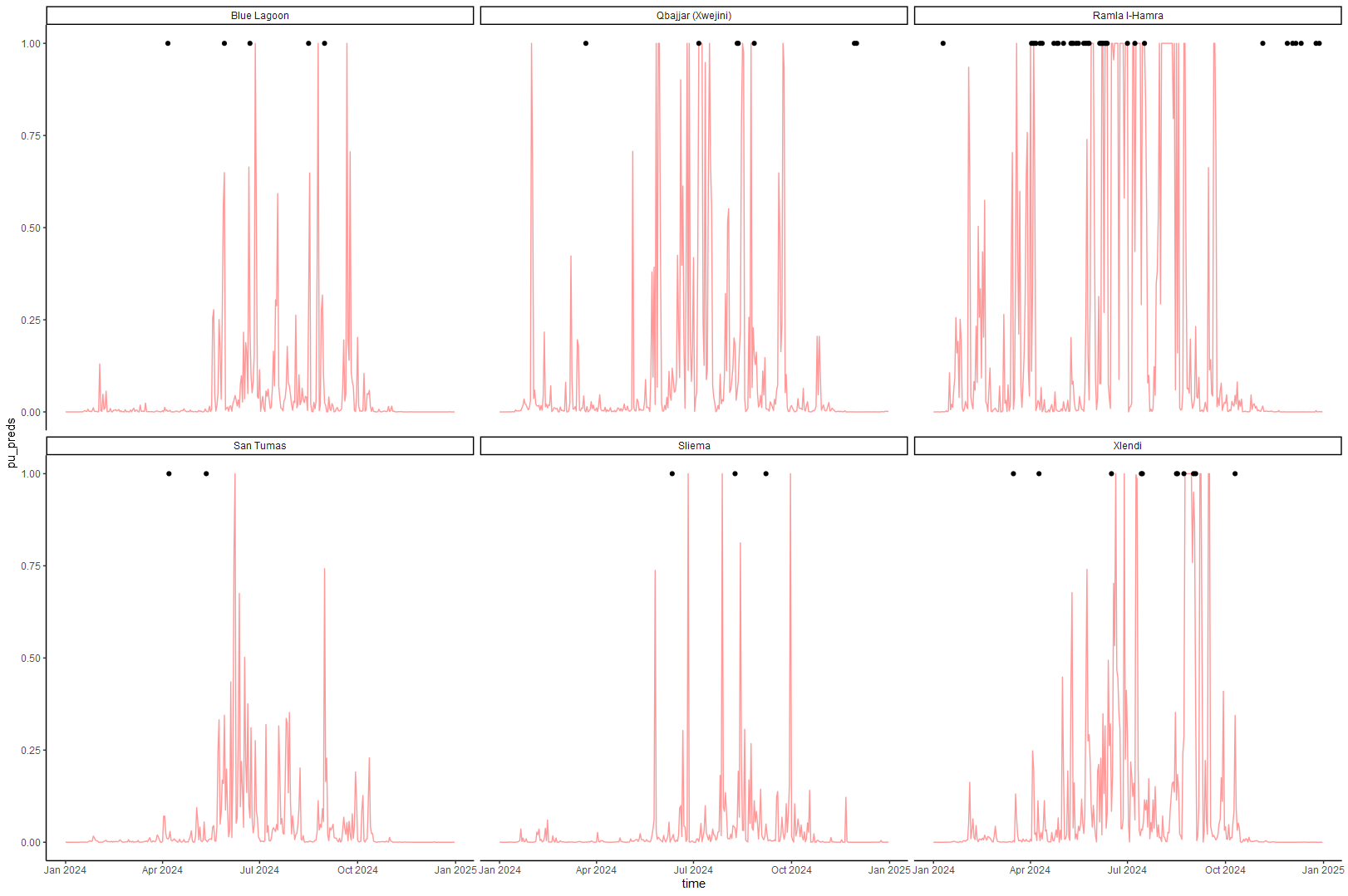
Lastly I glossed over the fact that “Positive Unlabled Data” is itself a topic of active machine learning research. One thing I did try was to incorporate a label frequency along the lines of this paper.
The ‘constant’ factor is what your initial model predicts on a holdout set of positive-only labels divided by the number of those positive examples.
Again, it works, just not as well as you would need to show this to people.
I also tried to constrain the problem to make it simpler, by for example only using summer months (this messed the neural network models where you would feed sequences) or labels with Pelagia noctuila only (this is the most commonly observed jellyfish in Malta, about half of all labels).
Other experiments
Something else I tried was to ensemble a variety of the above together in creative ways. For instance in some of the PU literature one thing that professional ecologists would do is use a MaxEnt model to generate “presence weights” and use this as an input to subsequent models.
Another hybrid approach I tried was a much leaner ML model for jellyfish prediction and then using opendrift to simulate beachings from n * this probability jellies. Indeed there is a certain logical niceness to decoupling the probability of a jellyfish bloom from the probability it will make a beaching and use separate models for each. James Cant has a great shinyapp with this set up here.
Other Steps I Considered But Didn’t Code Up
One of the advantages of neural networks is that they could in theory operate on the raw rasters. I never fully explored this, instead opting to feed these models my tabular data I had created for my other models.
In some ways I also “threw away” data from most of the raster cells: with 36 beach locations you end up using 36 cells out of the ~460 that cover the extent for Malta I was using. At times I had a nagging suspicion there was good signal in adjacent cells I was missing that something like a Graph Neural Network could tap into.
What’s next?
I’m not too sure. I’ve been taking a break and coming back to this project a while, often just before summer. I might revisit it if I come across some new exciting approach that I suspect might help, but in lieu of that it will probably remain parked. My gut intuition is that the best improvements will come through more and better labels.
What I’ve also neglected to mention is that along the three years I’ve been sending a flurry of emails to any researcher who will listen. Many actually did, but my most helpful discussions were with Jairo Castro-Gutiérrez and Joe El Rahi, and I thank them for their time. I also can’t ever forget some random soul in the Catalan Water Agency who taking pity on my Google translated Catalan sent me a spreadsheet of all recorded beachings in the past year.
In the end, there is a certain poetic beauty in the fact that a jellyfish’s humble 10,000 neurons, scattered throughout its body and not part of any centralised nervous system, can result in such intricately complex and adaptable behaviour. A friend recently reminded me of Saint-Exupéry’s remark that “perfection is achieved, not when there is nothing more to add, but when there is nothing left to take away”, and my immediate thought was that by that metric, the jellyfish was perfect.
And perhaps, I should go down to the beach.