Who would have been elected if we had the gender reform bill in the past?

How does the Gender Quota Bill work?

The best explainer I could find on how the reform will work is from this public consultation document dated from March 2019. I’m not sure if the final version passed in Parliament is exactly identical.

In any case, the gist is in pages 41 to 47, where the process is proposed as:

1. Allow the usual election counting, constitutional adjustment and casual elections to take place as they currently do.

2. If two parties make it to parliament, calculate the proportion of MP’s by gender.

3. If one gender has less than 40% of the seats, trigger the clause.

4. Calculate the number of seats needed by the underrepresented gender to reach the 40% quota. Although the required seats to reach 40% might be more than 12, the maximum number of seats allocated can be 12, equally split between the parties.

5. Fill these seats using a ranked list that prioritizes candidates of the under-represented gender who suffered from “wasted” votes in their district. This is a bit more complex than one assumes at first, since two ways are proposed. The first is rank by left over votes that can’t be transferred once 5 MP’s are elected from a district - this seems straight forward. The second entails using the leftover votes of the over-represented gender and holding “casual” elections transferring these votes to the under-represented gender. We can’t do this using the summarized data.

6. If this list is exhausted, and seats remain available, parties can co-opt their choices.

The Data

Like in other projects, we’ll use the Malta Elections dataset originally started by Professor John C. Lane and currently hosted by the University of Malta. The data here spans from 1921 to 2013, allowing us to simulate all but the last legislature.

Step 1: Find in which Legislatures the Mechanism is applicable

For a legislature to be applicable it needs to have a gender imbalance of 60% and consist of only two parties. We can calculate those as follows:

library(readxl)
library(tidyverse)

elections <- read_excel("C:/Users/Charles Mercieca/Documents/RProjects/Parliament Gender Reform/Input/elections.xls")

prop_women <- elections %>% 
  filter(SEATED != 0,
         PARTY != 99) %>% 
  mutate(SEX = SEX-1) %>% 
  group_by(election = YEAR) %>% 
  summarise(proportion_women = mean(SEX))

parties <- elections %>%
  filter(WIN != 0,
         PARTY != 99) %>% 
  group_by(YEAR) %>% 
  distinct(PARTY) %>% 
  group_by(election = YEAR) %>% 
  tally(name = "Parties Elected to Parliament")

legislatures <- prop_women %>% 
  inner_join(parties) %>% 
  mutate(activate_mechanism = proportion_women < 0.4 &
           `Parties Elected to Parliament` == 2)

legislatures %>% tail(10)

## # A tibble: 10 x 4
##    election proportion_women `Parties Elected to Parliament` activate_mechanism
##       <dbl>            <dbl>                           <int> <lgl>             
##  1     1971           0.0357                               2 TRUE              
##  2     1976           0.0429                               2 TRUE              
##  3     1981           0.0290                               2 TRUE              
##  4     1987           0.0278                               2 TRUE              
##  5     1992           0.0145                               2 TRUE              
##  6     1996           0.0571                               2 TRUE              
##  7     1998           0.0909                               2 TRUE              
##  8     2003           0.0870                               2 TRUE              
##  9     2008           0.0870                               2 TRUE              
## 10     2013           0.130                                2 TRUE

The first condition always has been true for every General Election so far. Since women’s suffrage was only established in time for 1947 election, and before that no women contested, 6 legislatures spanning 1921-1945 are out.

The 1951, 1953 and 1962 elections also resulted in more than 2 parties being elected, which leaves us with 11 elections to play with.

ggplot(legislatures, aes(x = election, y = proportion_women))+
geom_line()+
geom_point(aes(col = activate_mechanism))+
scale_y_continuous(labels = scales::percent)+
  theme_light()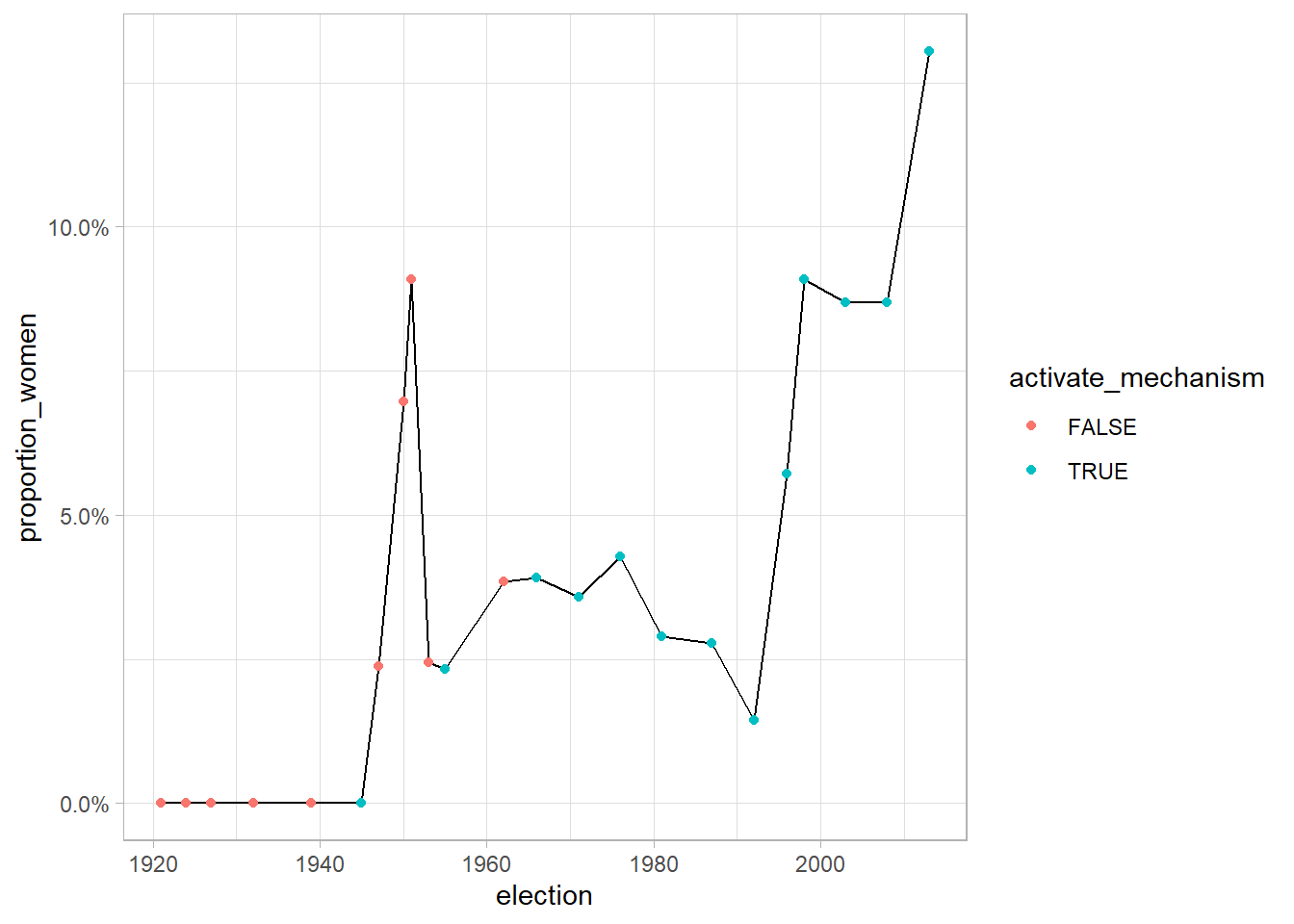

Step 2: Calculate Additional Seats

Slightly more involved is how to calculate the additional seats, which I’ve implemented in a function below following the maths from page 43 of the document.

additional_seats <- function(gender_under, gender_over){
  #Calculate extra seats to be added to Parliament
  additional_seats <- ((0.4 * gender_over) - gender_under) /
    0.6
  
  #Check to see that MP's remain an odd number and round down if not
  if (floor(additional_seats)+(gender_under+gender_over) / 2){
    floor(additional_seats) - 1
  }
  
  else {
    floor(additional_seats)
  }
}

The document also has two fictional scenarios with which we can test our function.

#Scenario 1: "the under-represented sex secured nine seats from a total of 67"..."x = 29.67 which is rounded down to 28"

additional_seats(9, 67) == 28

## [1] TRUE

#Scenario 2: "If the under-represented sex obtained 23 seats from a total of 69 seats, the total number of additional seats assigned to this under-represented group is 6"
additional_seats(23, 69) == 6

## [1] TRUE

Now we need to parse out how many men and women were elected or seated in casual elections throughout the legislatures, and then apply our function, accounting for the fact that if the maximum number of additional seats is limited to 12.

eligible_years <- legislatures %>% 
  filter(activate_mechanism == T,
         election >= 1947) %>% 
  pull(election)

seats <- elections %>% 
  filter(YEAR %in% eligible_years,
         SEATED != 0,
         PARTY != 99) %>%
  group_by(YEAR, SEX) %>% 
  tally() %>% 
  pivot_wider(names_from = SEX, values_from = n) %>% 
  rename(men = "1", women = "2") %>% 
  mutate(calculated_seats = additional_seats(women, men),
         adjusted_seats = if_else(calculated_seats > 12, 
                                  12, 
                                  calculated_seats))
seats

## # A tibble: 12 x 5
## # Groups:   YEAR [12]
##     YEAR   men women calculated_seats adjusted_seats
##    <dbl> <int> <int>            <dbl>          <dbl>
##  1  1955    42     1               25             12
##  2  1966    49     2               28             12
##  3  1971    54     2               31             12
##  4  1976    67     3               38             12
##  5  1981    67     2               40             12
##  6  1987    70     2               42             12
##  7  1992    68     1               42             12
##  8  1996    66     4               36             12
##  9  1998    60     6               29             12
## 10  2003    63     6               31             12
## 11  2008    63     6               31             12
## 12  2013    60     9               24             12

Step 3: Compile List

Now we need a fair way to fill those 12 seats. I did struggle to understand all the gist of the documentation here, but my understanding is the safest bets are “hanging” candidates of the minority gender.

It’s actually pretty trivial to calculated the “wasted” votes from our dataset, we just need to find candidates whose maximum count was equivalent to their last count like this:

wasted_votes <- elections %>% 
  filter(YEAR %in% eligible_years,
         SEATED == 0,
         TOPS == LAST,
         PARTY != 99)

w <- wasted_votes %>% 
  group_by(YEAR, Dist) %>% 
  summarise(max(LAST))

## `summarise()` has grouped output by 'YEAR'. You can override using the `.groups` argument.

From here I thought it was fairly straightforward: find these candidates, filter for the ones that are women and we’d have most of the list. But it turns out that only three of those candidates with wasted votes are women.

wasted_votes %>% 
  filter(SEX == 2) %>% 
  select(YEAR, NAME, Dist)

## # A tibble: 3 x 3
##    YEAR NAME           Dist
##   <dbl> <chr>         <dbl>
## 1  2003 Law, Rita         2
## 2  2008 Dalli, Helena     3
## 3  2008 Law, Rita         3

Which is probably why the document mentions that vote transferring mechanism. But given the document doesn’t delve too deeply into the details here and reverse engineering transfers might be too bold of an undertaking for a weekend project, the below is a rough approximation using the highest votes a candidate saw (i.e. the TOPS variable).

For the 1st elected candidate in a district, this will be the first count, for the 2nd elected the second and so on. Since by default the candidates we’re looking into were not elected, higher TOPS counts indicate a higher preference to transfer votes to that candidate.

#Create filter list for candidates elected in other districts in same year (e.g. Claudette Buttigieg in 2013)

elected_seperately <- elections %>% 
  filter(SEATED != 0) %>% 
  distinct(YEAR, NAME)

#Select best performing women among non-elected candidates nation wide
candidates <- elections %>% 
  filter(YEAR %in% eligible_years,
         SEATED == 0, #Filter out elects, including adjustment and casual elec.
         PARTY %in% c(13, 15), #PN & PL
         SEX == 2) %>%  #Women
  mutate(PARTY = case_when(PARTY == "13" ~ "PL",
                           PARTY == "15" ~ "PN")) %>%
  anti_join(elected_seperately) %>% 
  select(YEAR, NAME, PARTY, Dist, CT1, TOPS) %>% 
  group_by(YEAR, PARTY, Dist) %>% 
  arrange(YEAR, PARTY, desc(TOPS)) %>% 
  group_by(YEAR, PARTY) %>% 
  slice(1:6) %>% 
  mutate(YEAR = as.factor(YEAR),
         PARTY = as.factor(PARTY)) %>% 
  arrange(desc(YEAR))

## Joining, by = c("NAME", "YEAR")

We can pipe this into an interactive HTML table using the DT package:

library(DT)
library(widgetframe)

table <- datatable(candidates, filter = 'top', options = list(
  pageLength = 24, autoWidth = TRUE))

widgetframe::frameWidget(table)

Or alternatively:

ggplot(candidates, aes(fct_reorder(NAME, TOPS), TOPS, fill = PARTY))+
  geom_col()+
  coord_flip()+
  facet_wrap(~YEAR, 
             scales = "free", 
             ncol = 2)+
  ylab("Highest Vote Count Candidate Achieved Before Transfer")+
  xlab("")+
  theme_light()+
  theme(legend.position="top")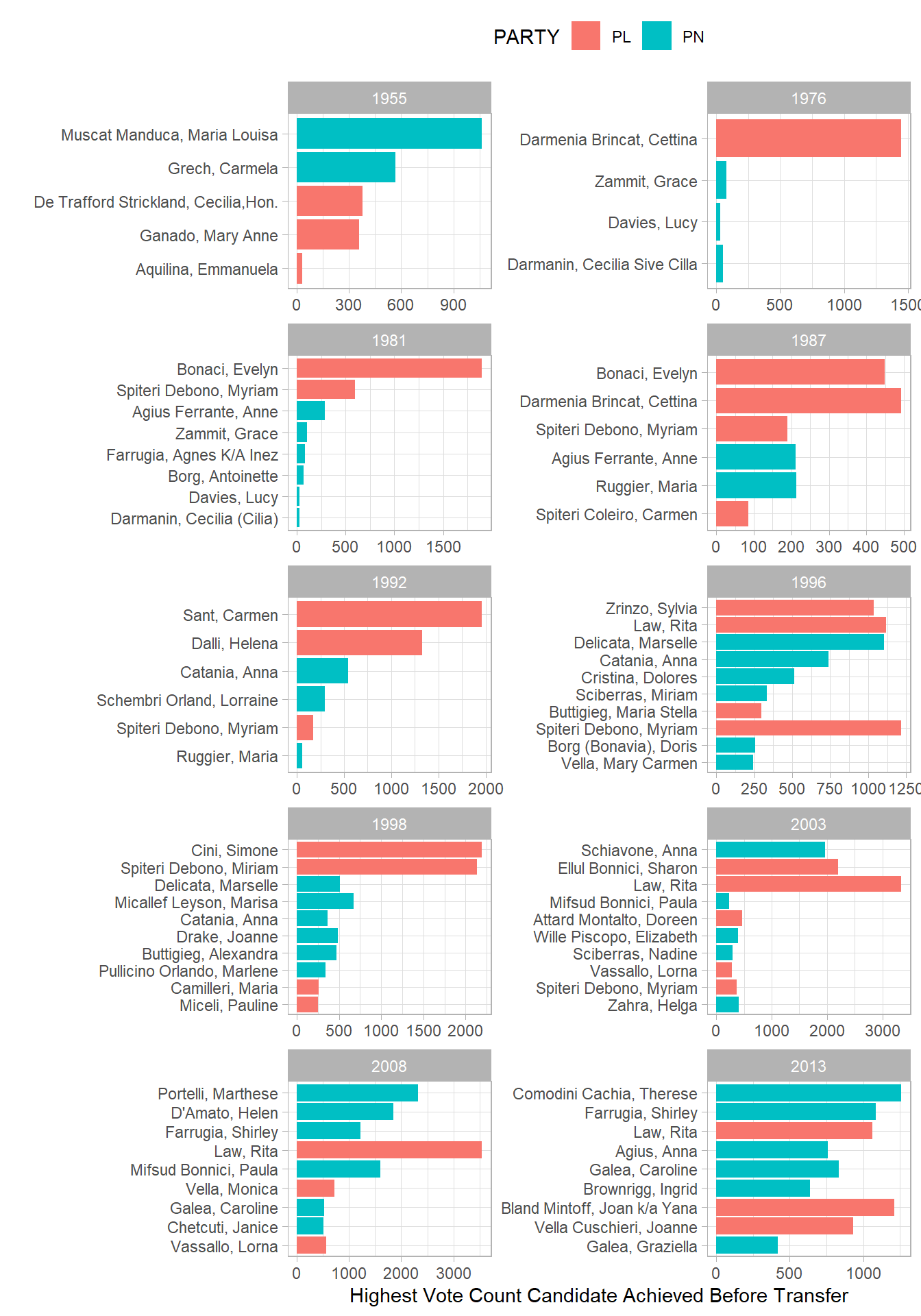

We stumble into two areas of added complexity here:

1. Sometimes the adjustment downward to ensure an odd overall parliament will result in an odd list (i.e. 11 candidates) How would this be split among the two parties?

2. Well performing candidates perform well in multiple districts. Taking 2013 as an example, Yana Bland Mintoff, Rita Law and Joanne Vella Cuschieri all did well in two districts (hence we captured them twice). In some cases it would probably entail having casual elections of casual elections using the results of casual elections, which are several orders of abstractions above the result on election day.

Interestingly, a number of politicians that would have of made it to Parliament are those that did eventually make it in future years: Therese Comodini Cachia in 2013 (elected in 2017), Paula Mifsud Bonnici and Marthese Portelli in 2008 (both elected in 2013), Marlene Farrugia in 1998 and Helena Dalli in 1992 (subsequently elected in 1996).

Another noteworthy instance is in the case of Rita Law, where the mechanism would mean that someone who made it to Parliament in 1998 but subsequently did not despite relatively solid performances would have of returned to the MP benches.

As an aside, one of the 1955 candidates that would have of made it is Cecilia Strickland, sister of Mabel and daughter of Gerald, who eventually left Malta and settled in Surrey.