Spend and Votes in the 2019 MEP Election

Looking at Just Spend vs Votes

Now I had already done something similar to this before for the 2017 General Election, but in that case only candidates that got elected declared their spend. So while it was clear that candidates who spent more got more votes, we can’t say this is true for all candidates. In this way, this analysis will be more rigorous because we have the spend of the whole field of candidates, regardless of the outcome.

And sure enough, when you plot it, the relationship between spend and votes is just as you’d expect: as one goes up, so does the other.

## `geom_smooth()` using formula 'y ~ x'

Fitting a linear model tells us that the average votes a candidate got was 1314, and that for every one euro of spend, a candidate gets an additional 0.47 of a vote, or 2.12 euros per vote.

lm(FirstCountVotes~Spend, data = MEPData) %>% 
summary()

## 
## Call:
## lm(formula = FirstCountVotes ~ Spend, data = MEPData)
## 
## Residuals:
##    Min     1Q Median     3Q    Max 
## -16882  -2419  -1207   -208  49630 
## 
## Coefficients:
##              Estimate Std. Error t value Pr(>|t|)    
## (Intercept) 1314.4216  2120.9299   0.620 0.539228    
## Spend          0.4721     0.1142   4.133 0.000197 ***
## ---
## Signif. codes:  0 '***' 0.001 '**' 0.01 '*' 0.05 '.' 0.1 ' ' 1
## 
## Residual standard error: 10500 on 37 degrees of freedom
## Multiple R-squared:  0.3158, Adjusted R-squared:  0.2974 
## F-statistic: 17.08 on 1 and 37 DF,  p-value: 0.0001968

Not a bad start! However we’re only explaining around 30% of the variance up to this point.

Adding Facebook likes

What if we add Facebook Likes? Visualising them like before, they also look like a strong predictor:

## `geom_smooth()` using formula 'y ~ x'

## Warning: Removed 7 rows containing non-finite values (stat_smooth).

## 
## Call:
## lm(formula = FirstCountVotes ~ Spend + FacebookLikes, data = MEPData)
## 
## Residuals:
##    Min     1Q Median     3Q    Max 
## -11678  -2019   1146   1840  14554 
## 
## Coefficients:
##                 Estimate Std. Error t value Pr(>|t|)    
## (Intercept)   -1.354e+03  1.097e+03  -1.234   0.2252    
## Spend         -1.383e-01  8.180e-02  -1.691   0.0995 .  
## FacebookLikes  1.023e+00  9.754e-02  10.491  1.7e-12 ***
## ---
## Signif. codes:  0 '***' 0.001 '**' 0.01 '*' 0.05 '.' 0.1 ' ' 1
## 
## Residual standard error: 5286 on 36 degrees of freedom
## Multiple R-squared:  0.8314, Adjusted R-squared:  0.822 
## F-statistic: 88.74 on 2 and 36 DF,  p-value: 1.215e-14

But something weird happens as soon as we add Facebook likes to the linear model. The R-Squared jumps up to 80%, indicating we’re accounting for much more of the variance than before. But spend is now negatively associated with votes, and we were seeing just the opposite before. The intercept has also changed dramatically.

Multicollinearity

Linear models expect independent variables to be, well, independent. And it turns out that Spend and Facebook likes are very strongly correlated:

cor(MEPData$Spend, MEPData$FacebookLikes)

## [1] 0.7113364

What this tells us is that those variables seem to be measuring the same concept. It could for instance be the case that the more popular a candidate is, the easier it becomes to acquire funds to spend, and the more followers on Facebook one gets as a result of this advertising.

Feeding our model two highly correlated variables makes us run into a problem called multicollinearity. Now if our aim was to make predictions of a candidate’s first count votes given spend and Facebook likes, this wouldn’t be a problem. After all, it’s improved the goodness of the fit of the model by 50%. But given that we’re more interested in explaining the presence and size of effects, we need to address it.

Given that we’ve already seen how cost alone is associated with votes, let’s take the easy way out and remove cost for now, and add the effect of incumbency:

lm(FirstCountVotes ~ FacebookLikes + Incumbent, data = MEPData) %>% 
  summary()

## 
## Call:
## lm(formula = FirstCountVotes ~ FacebookLikes + Incumbent, data = MEPData)
## 
## Residuals:
##      Min       1Q   Median       3Q      Max 
## -11178.4  -2424.7    309.7   1728.8  17632.4 
## 
## Coefficients:
##                 Estimate Std. Error t value Pr(>|t|)    
## (Intercept)   -1450.2727  1098.9276  -1.320    0.195    
## FacebookLikes     0.7862     0.1057   7.438 8.81e-09 ***
## IncumbentY     5843.4895  3903.2622   1.497    0.143    
## ---
## Signif. codes:  0 '***' 0.001 '**' 0.01 '*' 0.05 '.' 0.1 ' ' 1
## 
## Residual standard error: 5328 on 36 degrees of freedom
## Multiple R-squared:  0.8286, Adjusted R-squared:  0.8191 
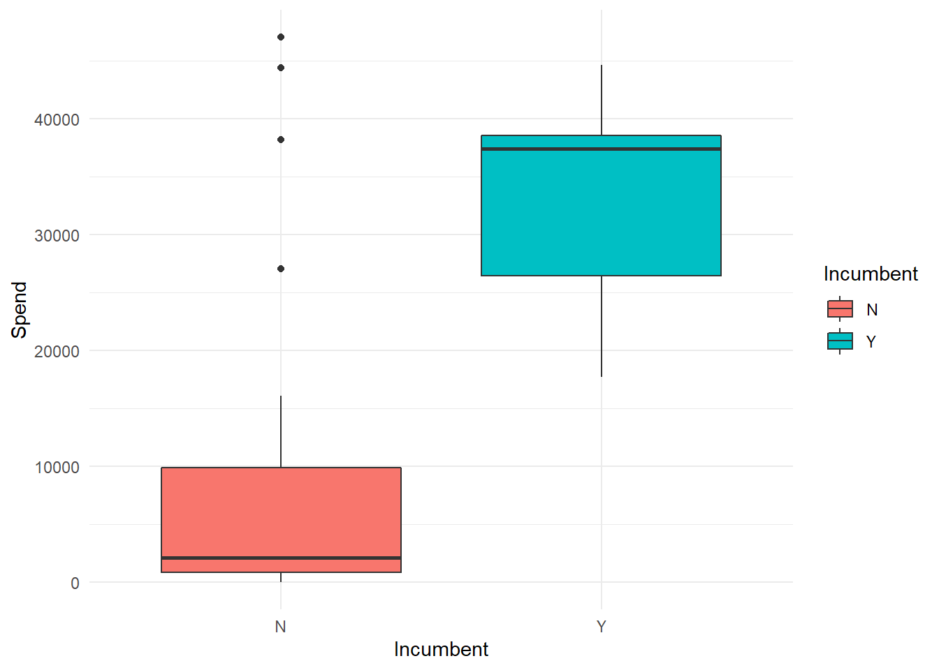
## F-statistic: 87.04 on 2 and 36 DF,  p-value: 1.622e-14

Surprisingly, Facebook likes seem to be an even better predictor of first count votes than spend. And as expected, already being an MEP is a huge advantage, with our model saying it’s worth an additional 5843 votes. Whether this popularity is because incumbents have access to more financing or if this higher access to financing is because of popularity is a chicken and egg question, but incumbents spent a median of 37,438 euros in the 2019 campaign as opposed to a median of 2,117 by non-incumbents.

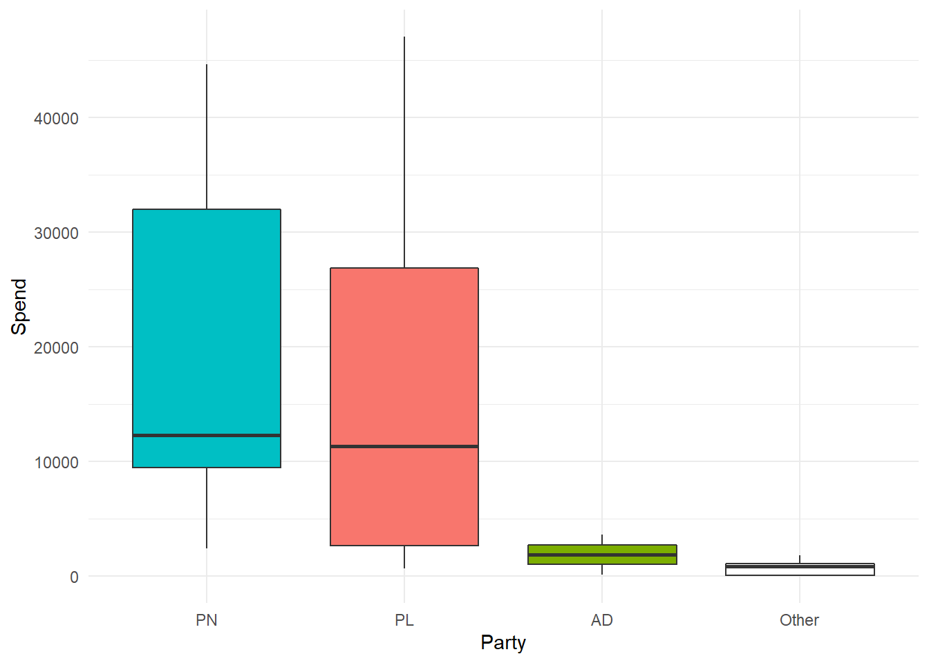
Spend by Parties

The average PN MEP candidate also outspent the average PL candidate, and the two major parties comprise the bulk of the spend:

When it comes to social media however, one party does seem to have a disproportional success. PD’s median likes ae equal to PL’s and greater than PN’s, however both main parties have huge outliers over the 50K mark (Dalli & Metsola).

MEPData %>% mutate(Party = fct_lump(Party, n = 3, w = FacebookLikes)) %>% 
ggplot(aes(x = fct_reorder(Party, -FacebookLikes), y = FacebookLikes, fill = Party))+
  geom_boxplot()+
  scale_fill_manual(values=c("Orange", "#F8766D", "#00BFC4", "White"))+
  theme(legend.position = "none")+
  xlab("Party")+
  ylab("Number of Facebook Page Likes")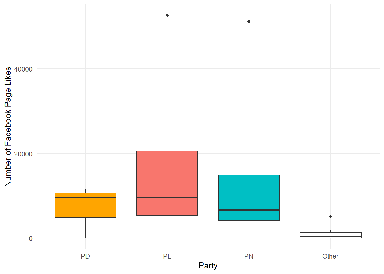

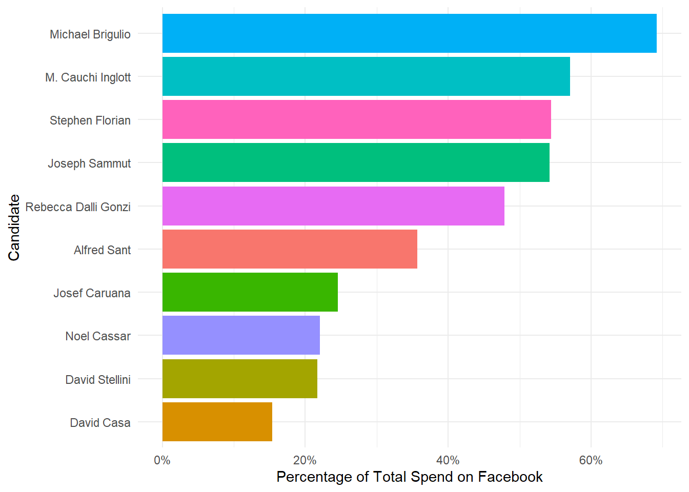
Spend on Digital?

So, what’s the ratio of money spent purely on Facebook out of the whole campaign? To do this, I just divided the amount spent on social media by the total amount declared to have of been spent. The candidates that had no social media spend were excluded. The top embracers of the digital world were:

The bottom 10 were:

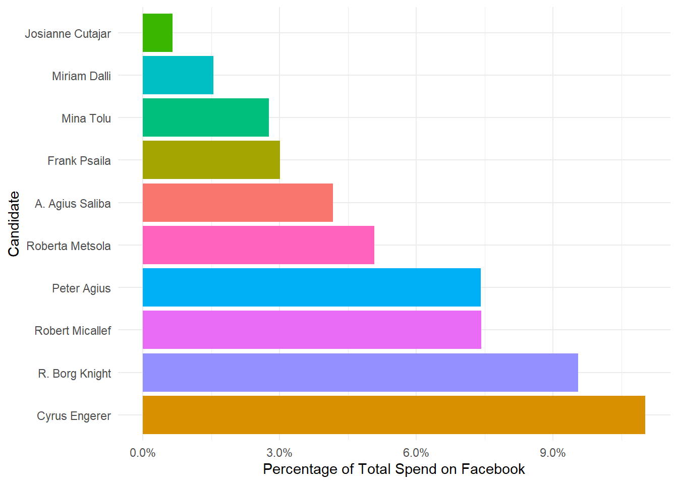
While it’s surprising to see heavyweights like Miriam Dalli, Josianna Cutajar and Roberta Metsola in this graph, it would be wise to keep in mind that those individual campaigns got significant boosts from their respective party’s main platform, which were declared seperately in the MaltaToday article.

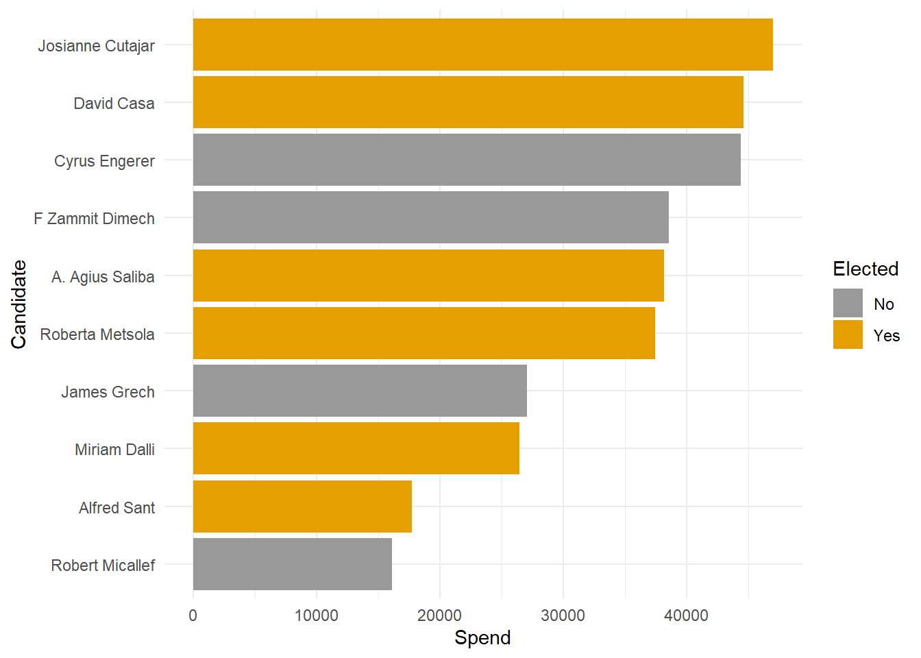
What have we learned?