New Esprimi Poll
Times of Malta/Esprimi came out with a new poll last weekend with some newer methodology than we’re used to. Though I have a feeling it largely made the rounds and captured the imagination of many because it bumped up the “40,000 lead” net figure to “50,000”. Percentage wise however, we’re bang on to other recent polls, in the 41% range for PN and 58% range for PL.
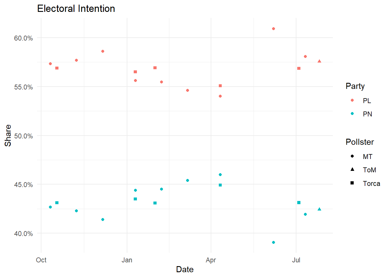
If you’re really pedantic, it’s actually a 0.5% improvement for PN from this MT poll around 3 weeks ago, and the emphasis on “number of votes” as opposed to % margin makes zero sense, but for many people it’s a bit like money at this stage: the more trailing zeros, the more excited they get.
Non Replies Issue
What it should really have of made the news about was on how differently it handled “no answer” responses. In European style polling, we usually readjust the denominator to the vote intention we have responses to, and rework that as a percentage out of 100 - implicitly assuming that the “no answers” are split along the same lines as the people that were vocal about it.
This is a fairly reasonable assumption unless you have reason to believe that the missingness is not at random but perhaps due to some sort of social desirability bias where supporters of an unorthodox party assess that their support is socially undesirable in the broader population.
(As a slight tangent, I said “European” style because in the US it’s perfectly normal to report a 40%-50% split as a ‘10 point lead’. In many ways this is actually a much more mature way to think about it.)
What Esprimi and Lobeslab have done is a step further: running a classification model on their responses and predicting the “no answer” category’s likely support.
In theory this approach should give similar results to weighing if the survey is properly designed, but I can see it possibly being a safeguard against some sort of survey wide bias. The catch here is however that this “bias” needs to be accounted for by some signal in the features (socially desirable non-responses are explained by for example location, to keep with the example) for machine learning techniques to pick it up.
The proof however, is always in practice.
Setting up our Experiment
If we synthetically create a population, and simulate sampling it just like a survey might, we can analyze the responses using traditional weighting vs. the machine learning approach. This would let us see if there is a meaningful difference of the estimated population values from the sample anf the true population value from our generated population.
Firstly, let’s write a function to generate our synthetic population:
create_population <- function(N = 500000,
                              blueberry_bias_age = 0,
                              blueberry_bias_location = 0){
  # Creates a sample population of blueberry & watermelon support
  #
  #       :param N(int): population size
  #       :param blueberry_bias_age(float): the bias in blueberry support according to age.
  #       :param blueberry_bias_location(float): bias in blueberry support according to location.

  #       :return (dataframe): composed of the synthetic population

set.seed(123)

  age_values <- c('18-30', '31-45',
                  '46-55', '56-65', '65+')
  age_probabilities <- c(0.13, 0.25, 0.15, 0.3, 0.17)

  region_value <- c('Gozitan Republic', 'Malta North',
                    'Malta West', 'Malta East', 'Malta South')
  region_probabilities <- c(0.1, 0.32, 0.1, 0.15, 0.33)

  population <- tibble(age = sample(age_values,
                                    N,
                                    prob = age_probabilities,
                                    replace = TRUE),
                       region = sample(region_value,
                                       N,
                                       prob = region_probabilities,
                                       replace = TRUE)) %>%
    mutate(preference = runif(nrow(.)),
           vote = case_when(age == '18-30' ~ preference + (blueberry_bias_age * 1.2),
                            age == '31-45' ~ preference + (blueberry_bias_age * 1),
                            age == '46-55' ~ preference,
                            age == '56-65' ~ preference - (blueberry_bias_age * 1),
                            age == '65+' ~ preference - (blueberry_bias_age * 1.5)),
           vote = case_when(region == "Malta North" ~ vote - blueberry_bias_location,
                            region == "Malta South" ~ vote + blueberry_bias_location,
                            TRUE ~ vote),
           vote = if_else(vote < 0.5, "Blueberry", "Watermelon")) %>%
    rowwise() %>%
    mutate(occupation = if_else(vote == "Blueberry",
                                sample(c("Farmer",
                                         "Office Work",
                                         "Healthcare",
                                         "Law Enforcment",
                                         "Bitcoin Trader",
                                         "Other"),
                                       1,
                                       replace = T,
                                       c(0.19, 0.16, 0.16, 0.16, 0.16, 0.17)),
                                sample(c("Farmer",
                                         "Office Work",
                                         "Healthcare",
                                         "Law Enforcment",
                                         "Bitcoin Trader",
                                         "Other"),
                                       1,
                                       replace = T,
                                       c(0.16, 0.17, 0.16, 0.16, 0.19, 0.16))),
           has_car = sample(c("Yes", "No"), 1, replace = T, c(0.5, 0.5))) %>%
    ungroup() %>%
    select(c("age", "region", "occupation", "has_car", "vote"))
}
create_population creates a Malta in an alternate reality, that’s exactly 500,000 people strong. Because this is in an alternate timeline, Gozo has achieved Republic status, but maintains strong social and economic ties with Malta. This is split into 4 regions, using the actual compass this time: North, West, East and South.
Rather than support for political parties, we’ll be measuring the nation’s favorite fruit: blueberry or watermelon. The blueberry_bias_age variable is important. If left to 0, the function will generate a random amount of support for both fruits. Over half a million rows, this will work out to nearly 50-50.
If tweaked with a positive value however, it will apply a bias in support, making blueberry less popular with younger groups, and more popular with older groups. If we want it to go another way, we can just apply a negative value.
Similarly, blueberry_bias_location works in much the same way, however in this case the bias is only applied to the Northern and Southern Malta regions.
To add some more predicting power, I created an occupation variable that’s slightly more farmer than chance if you like blueberries, and slightly more bitcoin trader if you like watermelons. The other has_car variable is just some random noise.
Creating Alternate Malta
All that’s left for us to create this alternate reality is to run the function!
set.seed(123)

malta_v2 <- create_population(blueberry_bias_age = 0.1,
                              blueberry_bias_location = 0.05)
Here, I’ll be biasing blueberry just a nudge with age (blueberry increases in popularity with age) and location (people in the north like to sprinkle them in yogurt for breakfast).
Anyway, the alternate Malta NSO’s latest census shows the population is comprised of:
census <- malta_v2 %>%
  group_by(age, region, occupation, has_car) %>%
  tally()

census
## # A tibble: 300 x 5
## # Groups: age, region, occupation [150]
## age region occupation has_car n
## <chr> <chr> <chr> <chr> <int>
## 1 18-30 Gozitan Republic Bitcoin Trader No 612
## 2 18-30 Gozitan Republic Bitcoin Trader Yes 582
## 3 18-30 Gozitan Republic Farmer No 539
## 4 18-30 Gozitan Republic Farmer Yes 586
## 5 18-30 Gozitan Republic Healthcare No 516
## 6 18-30 Gozitan Republic Healthcare Yes 520
## 7 18-30 Gozitan Republic Law Enforcment No 518
## 8 18-30 Gozitan Republic Law Enforcment Yes 540
## 9 18-30 Gozitan Republic Office Work No 527
## 10 18-30 Gozitan Republic Office Work Yes 541
## # ... with 290 more rowsThis is important because we’ll use this census to weigh our survey. Since we’re on the subject, here’s what the true support of blueberry vs. watermelon is in the population:
malta_v2 %>%
  group_by(vote) %>%
  summarise(n(), percent = n()/500000)
## # A tibble: 2 x 3
## vote `n()` percent
## <chr> <int> <dbl>
## 1 Blueberry 257031 0.514
## 2 Watermelon 242969 0.486And here’s the interaction by age and region:
malta_v2 %>%
  mutate(likes_blueberry = if_else(vote == "Blueberry", 1, 0)) %>%
  group_by(age, region) %>%
  summarise(blueberry_support = mean(likes_blueberry)) %>%
  ggplot(aes(x = region, y = blueberry_support, fill = age))+
  geom_col(position = "dodge")+
  coord_flip()+
  scale_y_continuous(labels = scales::percent)+
  theme_bw()+
  ylab("Blueberry Support")+
  xlab("")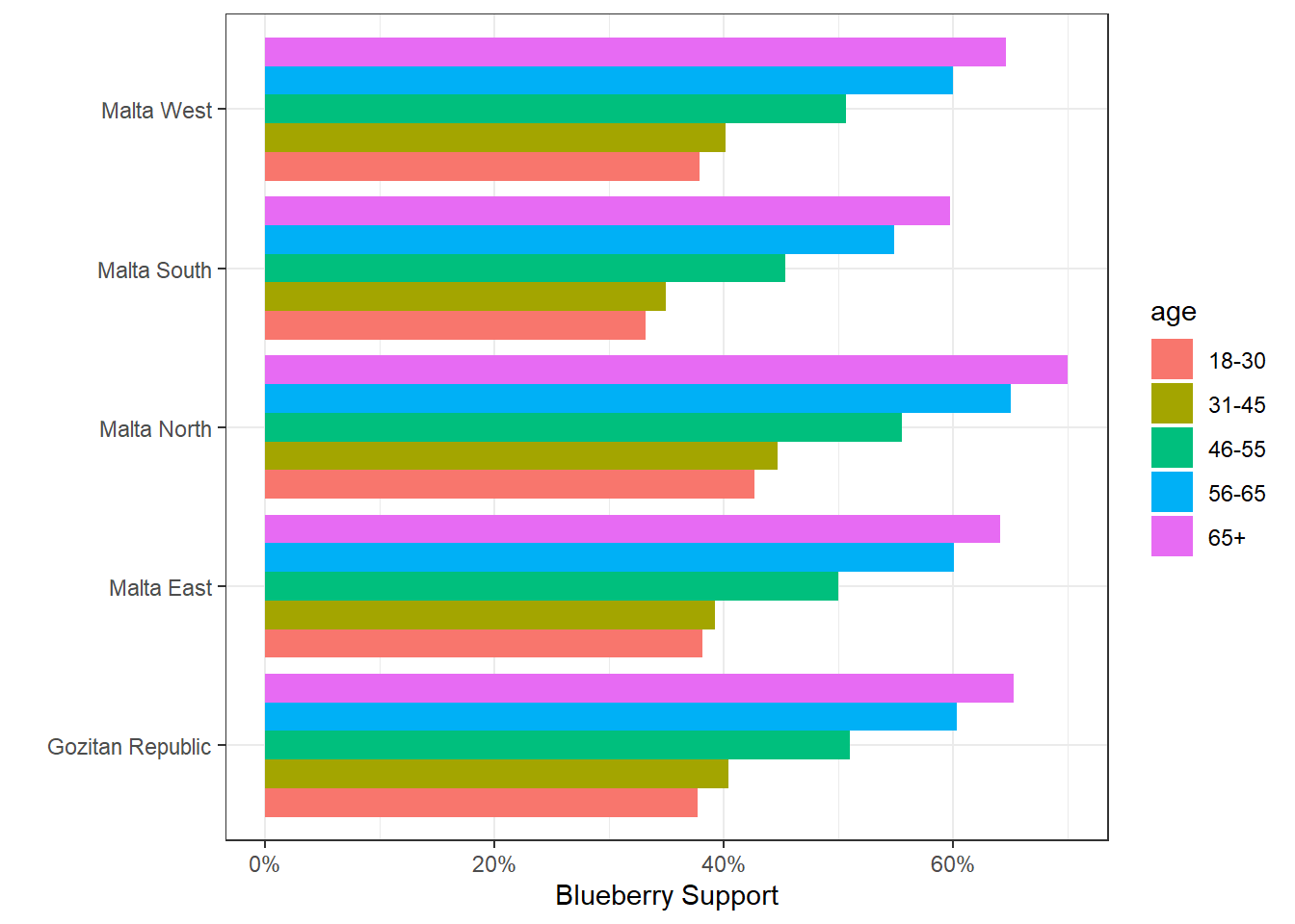
Our Survey
Similarly, we’ll wrap our survey in a function named survey_population.
survey_population <- function(population_df,
                              n = 600,
                              perc_shy = 0.1) {

  # Surveys the population randomly just like a phone survey might
  #
  #       :param population_df(dataframe): a population dataframe created using the create_population function.
  #       :param n(int): sample size
  #       :param perc_shy(float): the percentage of survey responses that will have 'no answer'

  #       :return (dataframe): the survey results
set.seed(234)
sample_n(population_df, replace = F, size = n) %>%
mutate(vote =  replace(vote,
                       sample(row_number(),
                              size = ceiling(perc_shy * n()),
                              replace = FALSE),
                       NA))
  }
The sample package’s sample_n actually does most of the heavy lifting here, but I added a line in a mutate call that randomly replaces the watermelon/blueberry value with an NA to simulate a stipulated percent of missing values. MaltaToday reports around 12-15% of “Don’t Knows”, so we’ll go with 15%, and generate a simulated survey of 600 people.
survey <- survey_population(malta_v2, n = 600, perc_shy = 0.15)This is what we get:
survey %>% head()## age region occupation has_car vote
## 1 31-45 Malta North Farmer No Watermelon
## 2 18-30 Malta East Bitcoin Trader Yes Blueberry
## 3 31-45 Malta South Healthcare Yes Watermelon
## 4 65+ Malta North Law Enforcment Yes <NA>
## 5 56-65 Malta South Other No Blueberry
## 6 31-45 Malta North Bitcoin Trader No <NA>And this is the picture our raw crosstabs paint:
survey %>%
  group_by(vote) %>%
  summarise(n(), n()/600)
## # A tibble: 3 x 3
## vote `n()` `n()/600`
## <chr> <int> <dbl>
## 1 Blueberry 254 0.423
## 2 Watermelon 256 0.427
## 3 <NA> 90 0.15Excitingly, due to the magic of randomness, watermelon is leading!
Traditional Surveys
The survey package is a tremendous resource in R for analysis. To make our lives easier, let’s join the census data to the survey. The pw column simply contains the number of that demographic group present in the population, while the fpc is the finite population correction, which we set to our 500,000 inhabitants.
library(survey)

survey_w_weights <- survey %>%
  inner_join(census) %>%
  rename(pw = n) %>%
  mutate(fpc = 500000)

survey_w_weights %>% head()
## age region occupation has_car vote pw fpc
## 1 31-45 Malta North Farmer No Watermelon 3422 5e+05
## 2 18-30 Malta East Bitcoin Trader Yes Blueberry 852 5e+05
## 3 31-45 Malta South Healthcare Yes Watermelon 3327 5e+05
## 4 65+ Malta North Law Enforcment Yes <NA> 2097 5e+05
## 5 56-65 Malta South Other No Blueberry 4013 5e+05
## 6 31-45 Malta North Bitcoin Trader No <NA> 3553 5e+05Then we can create our survey design object, and pass it through the svymean funtion.
design <- svydesign(id = ~1,
                    weights = ~pw,
                    data = survey_w_weights,
                    fpc = ~fpc)

svymean(~vote, design, na.rm = T)
## mean SE
## voteBlueberry 0.50918 0.0246
## voteWatermelon 0.49082 0.0246And what do you know, already a terrific improvement!
We’ve corrected the swing, and the true population value is within the standard error.
Classifier Aided
We can train a classification model on our provided survey responses, and use this to predict on the unknown responses. We’ll try two types of model: XGBoost and logistic regression from the glmnet package.
Julia Silge also introduced the finetune package in this video, so I also took this opportunity to give it a try. The pre-processing steps are pretty straight forward (some of it is actually copy pasted from the above video), but we’ll drop the NAs, create our folds, onehot encode all the predictors and give each of the models a 50 parameter grid, before analyzing performance on the unseen test set using the last_fit function.
XGBoost
library(tidymodels)
library(finetune)

doParallel::registerDoParallel()

set.seed(123)

raw <- survey %>%
  drop_na() %>%
  initial_split(0.8)

training <- training(raw)
testing <- testing(raw)

cv_folds <- vfold_cv(training)

classifying_rec <- recipe(vote ~ .,
                          data = training) %>%
  step_dummy(all_nominal_predictors(), one_hot = TRUE)

xgb_spec <-
  boost_tree(
    trees = 500,
    min_n = tune(),
    mtry = tune(),
    learn_rate = tune()
  ) %>%
  set_engine("xgboost") %>%
  set_mode("classification")

xgb_wf <- workflow(classifying_rec, xgb_spec)

xgb_rs <- tune_race_anova(
  xgb_wf,
  resamples = cv_folds,
  grid = 50)
xgb_last <- xgb_wf %>%
finalize_workflow(select_best(xgb_rs)) %>%
last_fit(raw)
xgb_last$.metrics## [[1]]
## # A tibble: 2 x 4
## .metric .estimator .estimate .config
## <chr> <chr> <dbl> <chr>
## 1 accuracy binary 0.480 Preprocessor1_Model1
## 2 roc_auc binary 0.530 Preprocessor1_Model1GLMNet
set.seed(234)

log_reg_spec <- logistic_reg(
  penalty = tune(),
  mixture = tune()) %>%
  set_mode("classification") %>%
  set_engine("glmnet")

lr_wf <- workflow(classifying_rec, log_reg_spec)

lr_rs <- tune_race_anova(
  lr_wf,
  resamples = cv_folds,
  grid = 50)

lr_last <- lr_wf %>%
  finalize_workflow(select_best(lr_rs)) %>%
  last_fit(raw)

lr_last$.metrics
## [[1]]
## # A tibble: 2 x 4
## .metric .estimator .estimate .config
## <chr> <chr> <dbl> <chr>
## 1 accuracy binary 0.520 Preprocessor1_Model1
## 2 roc_auc binary 0.543 Preprocessor1_Model1Now to be honest, both these models have dreadful performance. It may be entirely due to my synthetic data or something obvious I missed. But since the logistic classifier is a smudge better, let’s use that to predict the “unknowns” present in the survey.
lr_preds <- lr_wf %>%
  finalize_workflow(select_best(lr_rs)) %>%
  fit(training) %>%
  predict(survey)

survey_model_assist <- survey %>%
  bind_cols(lr_preds) %>%
  mutate(vote = case_when(is.na(vote)~ as.character(.pred_class),
                          TRUE ~ vote))
Raw
How well did it improve things from the raw results?
survey_model_assist %>%
  group_by(vote) %>%
  summarise(n(), n()/600)
## # A tibble: 2 x 3
## vote `n()` `n()/600`
## <chr> <int> <dbl>
## 1 Blueberry 298 0.497
## 2 Watermelon 302 0.503It swung 0.1% the wrong way.
As an Input to a Weighted Survey
But if we use that raw survey as the input to the usual weighing process…
survey_model_assist <- survey_model_assist %>%
  inner_join(census) %>%
  rename(pw = n) %>%
  mutate(fpc = 500000)
## Joining, by = c("age", "region", "occupation", "has_car")design_2 <- svydesign(id = ~1,
weights = ~pw,
data = survey_model_assist,
fpc = ~fpc)
svymean(~vote, design_2, na.rm = T)## mean SE
## voteBlueberry 0.5176 0.0227
## voteWatermelon 0.4824 0.0227That’s actually the closest result of the lot. Obviously, the better work you do on the classification model, the better your result will look.
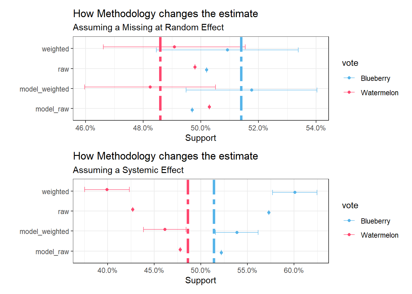
Summarizing It
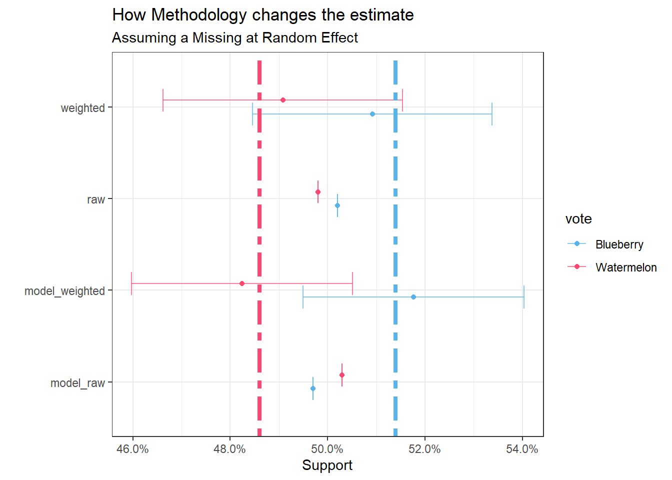
What if the Effect was systemic?
There’s one case where the ML approach might actually make a huge difference: if the missingness was not at random. To simulate this, I set the shyness to 0 (we get no NAs), order our table so the same categories are clustered together, and just chop off a bunch of let’s say, shy watermelon fans.
survey_biased <- survey_population(malta_v2, n = 600, perc_shy = 0) %>%
  arrange(vote, region, age) %>%
  head(510)
survey_biased %>%
group_by(vote) %>%
summarise(n()/510)## # A tibble: 2 x 2
## vote `n()/510`
## <chr> <dbl>
## 1 Blueberry 0.573
## 2 Watermelon 0.427Yikers. Now let’s do the same things.
survey_w_weights_2 <- survey_biased %>%
  inner_join(census) %>%
  rename(pw = n) %>%
  mutate(fpc = 500000)
## Joining, by = c("age", "region", "occupation", "has_car")design <- svydesign(id = ~1,
weights = ~pw,
data = survey_w_weights_2,
fpc = ~fpc)
svymean(~vote, design, na.rm = T)## mean SE
## voteBlueberry 0.60069 0.0239
## voteWatermelon 0.39931 0.0239In this case we can see that the weighing is way off. Pollsters will actually determine minimum respondents for each cell, but if it’s a systemic issue, some of those cells will remain empty.
set.seed(123)

raw <- survey_biased %>%
  drop_na() %>%
  initial_split(0.8)

training <- training(raw)
testing <- testing(raw)

cv_folds <- vfold_cv(training)

log_reg_spec <- logistic_reg(
  penalty = tune(),
  mixture = tune()) %>%
  set_mode("classification") %>%
  set_engine("glmnet")

lr_wf <- workflow(classifying_rec, log_reg_spec)

lr_rs <- tune_race_anova(
  lr_wf,
  resamples = cv_folds,
  grid = 50)

lr_last <- lr_wf %>%
  finalize_workflow(select_best(lr_rs)) %>%
  last_fit(raw)
## Warning: No value of `metric` was given; metric 'roc_auc' will be used.lr_last$.metrics## [[1]]
## # A tibble: 2 x 4
## .metric .estimator .estimate .config
## <chr> <chr> <dbl> <chr>
## 1 accuracy binary 0.618 Preprocessor1_Model1
## 2 roc_auc binary 0.674 Preprocessor1_Model1Interestingly, the logistic regression model’s performance jumps up: the missingness fit a pattern it’s learnt well.
lr_preds <- lr_wf %>%
  finalize_workflow(select_best(lr_rs)) %>%
  fit(training) %>%
  predict(survey)
## Warning: No value of `metric` was given; metric 'roc_auc' will be used.survey_model_assist <- survey %>%
bind_cols(lr_preds) %>%
mutate(vote = case_when(is.na(vote)~ as.character(.pred_class),
TRUE ~ vote))And in terms of raw and weighted numbers:
survey_model_assist %>%
  group_by(vote) %>%
  summarise(n(), n()/600)
## # A tibble: 2 x 3
## vote `n()` `n()/600`
## <chr> <int> <dbl>
## 1 Blueberry 313 0.522
## 2 Watermelon 287 0.478survey_model_assist <- survey_model_assist %>%
inner_join(census) %>%
rename(pw = n) %>%
mutate(fpc = 500000) ## Joining, by = c("age", "region", "occupation", "has_car")design_2 <- svydesign(id = ~1,
weights = ~pw,
data = survey_model_assist,
fpc = ~fpc)
svymean(~vote, design_2, na.rm = T)## mean SE
## voteBlueberry 0.53865 0.0227
## voteWatermelon 0.46135 0.0227Pretty cool!
Obligatory side by side tie-fighter plot for comparison:
library(patchwork)

plot_1 / plot_2