Campaign Spending

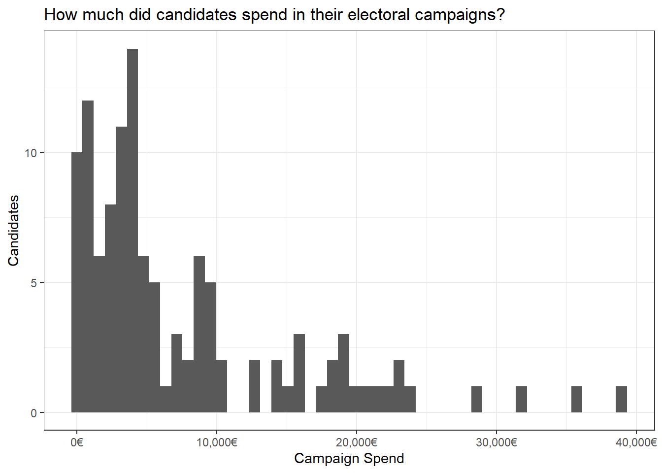
What’s the range of Campaign Spending?

Most candidates spent around 7,000 euros. Some however spent markedly less, and a handful spent upwards of 20,000 euros (median was 4,200).

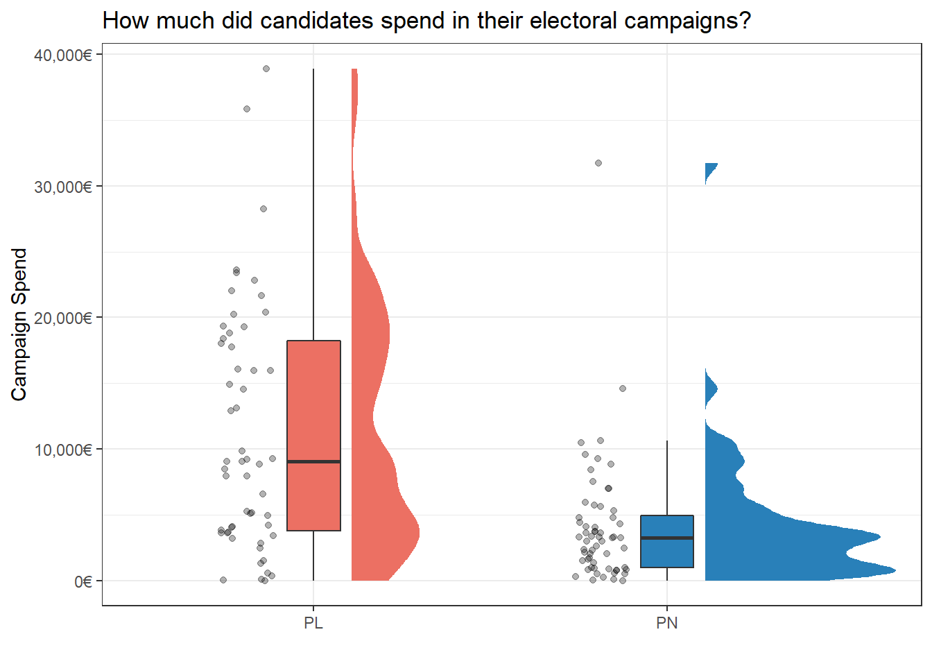
The average PL candidate spent more than the average PN candidate (p.s. see this post by Cédric Scherer on how to create these cool rainbow plots):

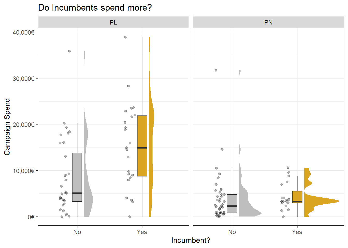
As did incumbent candidates. However this effect is much more pronounced for PL candidates than PN ones:

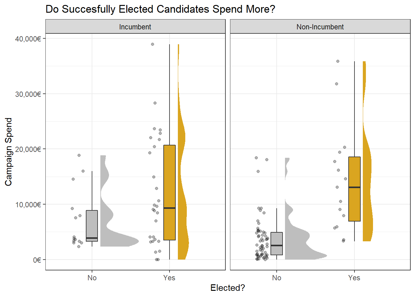
Do more expensive campaigns help you get elected more?

Perhaps the most important question to ask is if spending more means you get elected more. Although it seems so at first, reality might be more complicated. For example, we know incumbency is a powerful factor in getting elected, with politicians who were elected once before having an easier time making it again.

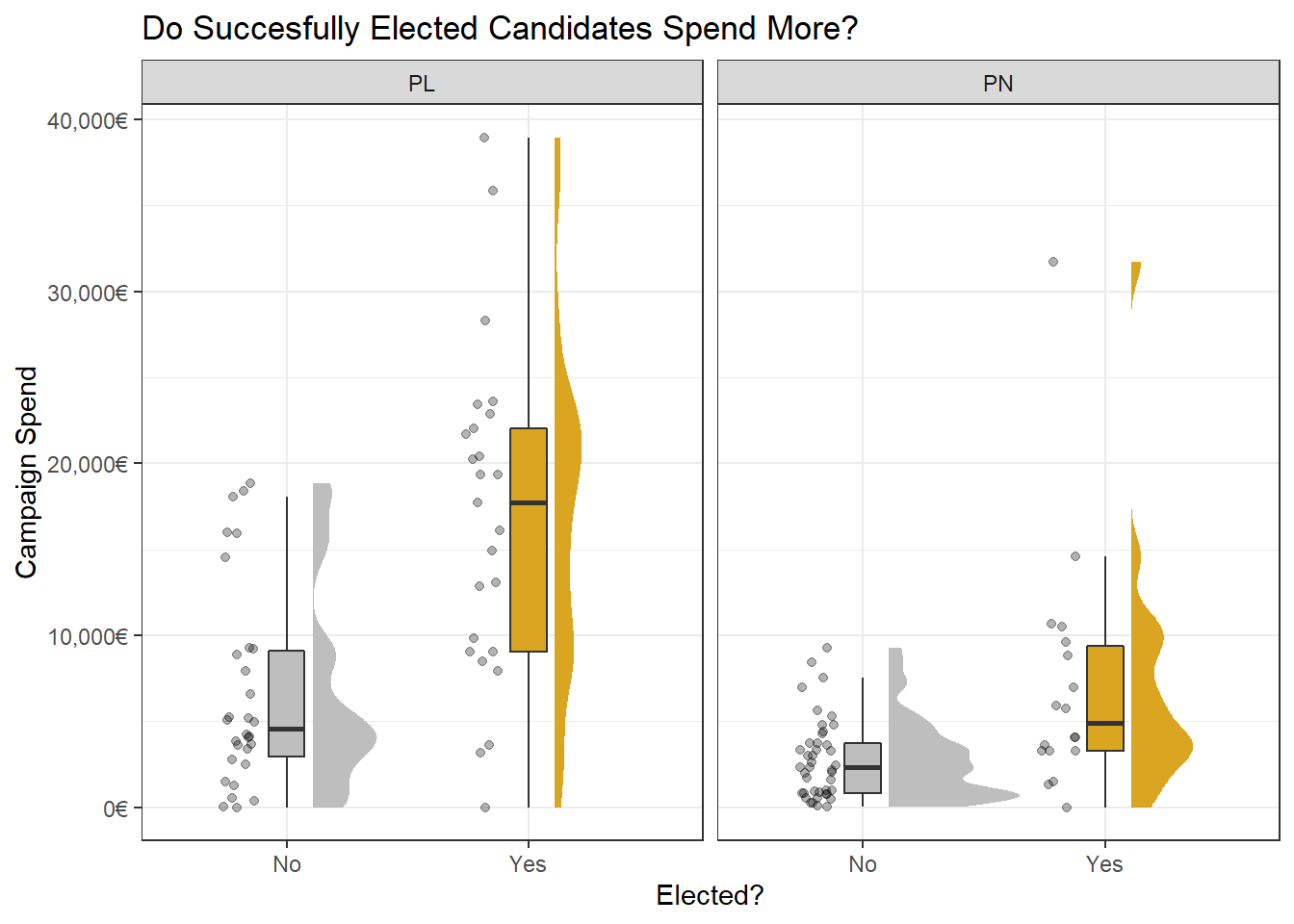
Some might argue that because of this, incumbents also have an easier time raising funds. The way to check for this is to split by incumbency. And the effect still stands, although it’s more pronounced with fresh non-incumbent candidates.

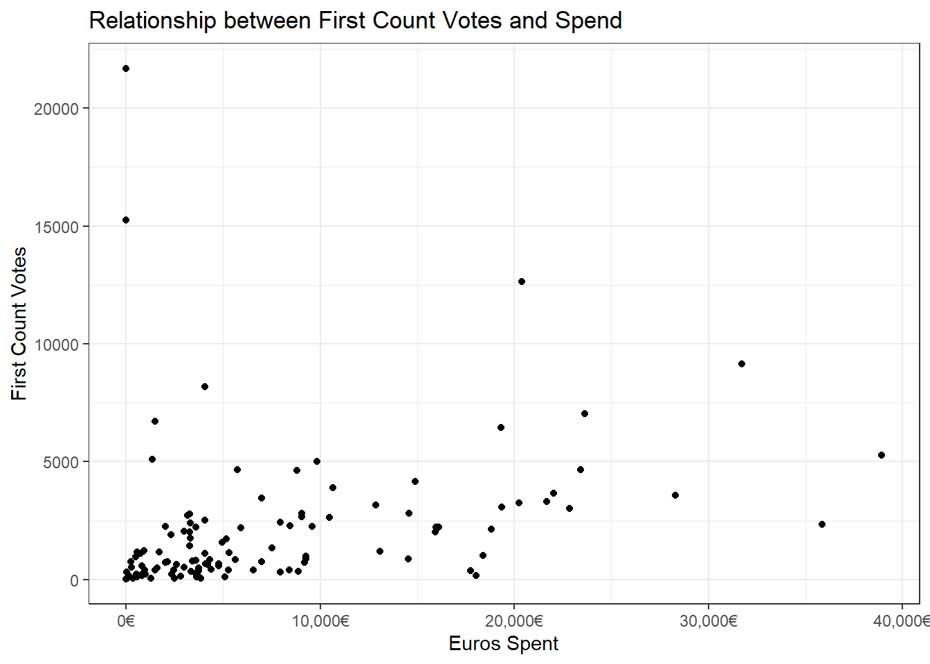
We can also plot the relationship between votes and spend. The most meaningful ones would be 1st count votes and last count, so let’s look at both.

The two high points at 0 euros of spend are Robert Abela and Bernard Grech, who customarily for leaders don’t have personal campaigns but piggyback on the party one. There does appear to be a weak relationship. The candidates that spent the least almost never got the most votes. And on the flipside those that spent the most didn’t get an enormous number of votes either, which points to a sweet spot of spend, beyond which returns are diminishing.

If we go for last count and filter out the two party leaders, we end up with something like this. Again, it’s weak but not exactly random.

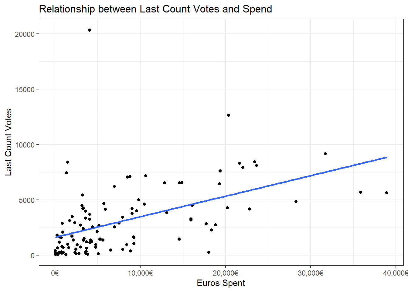
Or in more statistical terms, each additional euro spent adds 0.1 of a vote:

## 
## Call:
## lm(formula = count1_total ~ total_eur, data = .)
## 
## Residuals:
##     Min      1Q  Median      3Q     Max 
## -3045.6 -1284.3  -803.6   255.8 20360.3 
## 
## Coefficients:
##              Estimate Std. Error t value Pr(>|t|)    
## (Intercept) 1.330e+03  3.711e+02   3.583  0.00050 ***
## total_eur   1.051e-01  3.379e-02   3.109  0.00237 ** 
## ---
## Signif. codes:  0 '***' 0.001 '**' 0.01 '*' 0.05 '.' 0.1 ' ' 1
## 
## Residual standard error: 2926 on 114 degrees of freedom
## Multiple R-squared:  0.07814,    Adjusted R-squared:  0.07006 
## F-statistic: 9.664 on 1 and 114 DF,  p-value: 0.002374

Which Candidate got the most bang for their buck?

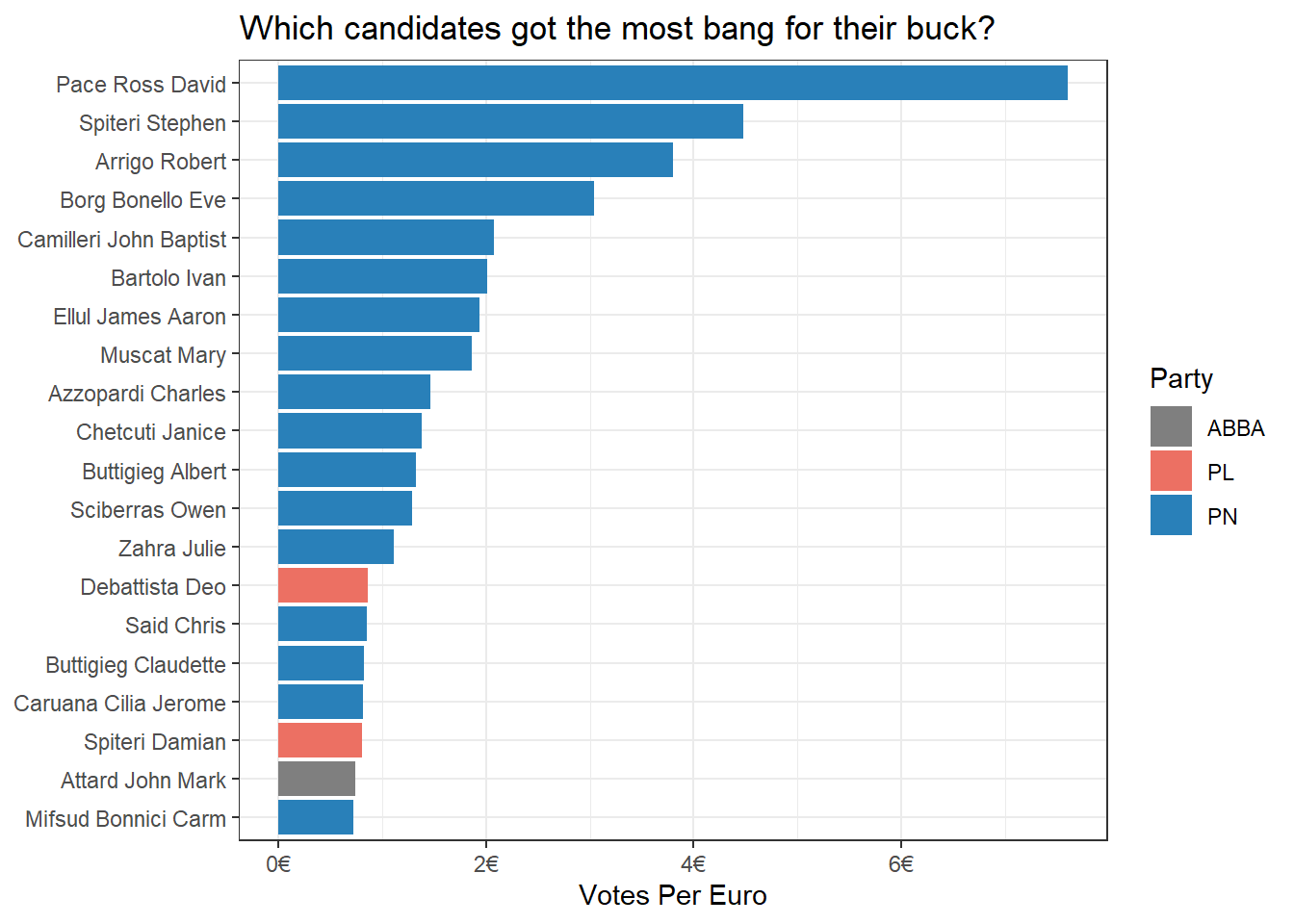
We can also come up with a ratio of which candidates got the most bang for their buck by calculating the ratio of votes to money spent:

Benford’s Law

Lastly we can check how close to expectations the declarations were. In 1938 Frank Benford noted that the leading digits of a range of numbers spanning a few orders of magnitude are distributed in a very characteristic way like this, with 1 being the leading digit 30% of the time and all other digits declining as a function of their rank.

The most intuitive explanation of why this happens is from this numberphile video, which explains that an 80 or a 90 needs only a tiny push to become a 100, but a 100 needs a relatively large push to become a 200 or 300.

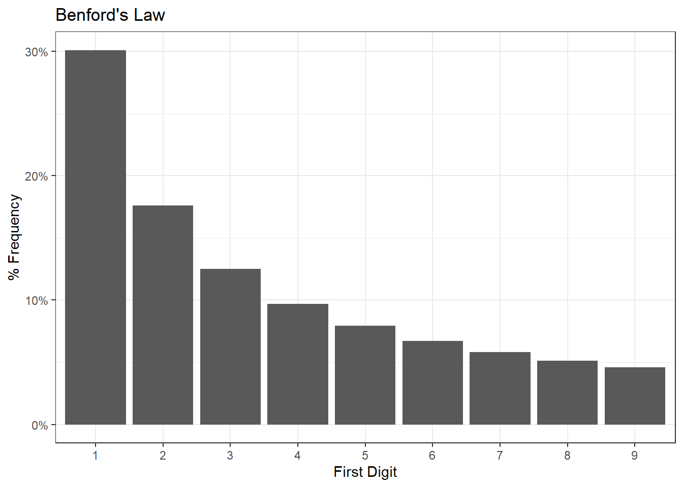
Benford’s law is used to catch all sorts of cooked numbers because humans often exhibit the inverse pattern when fudging, that is, rounding 1,020 down to say 950.

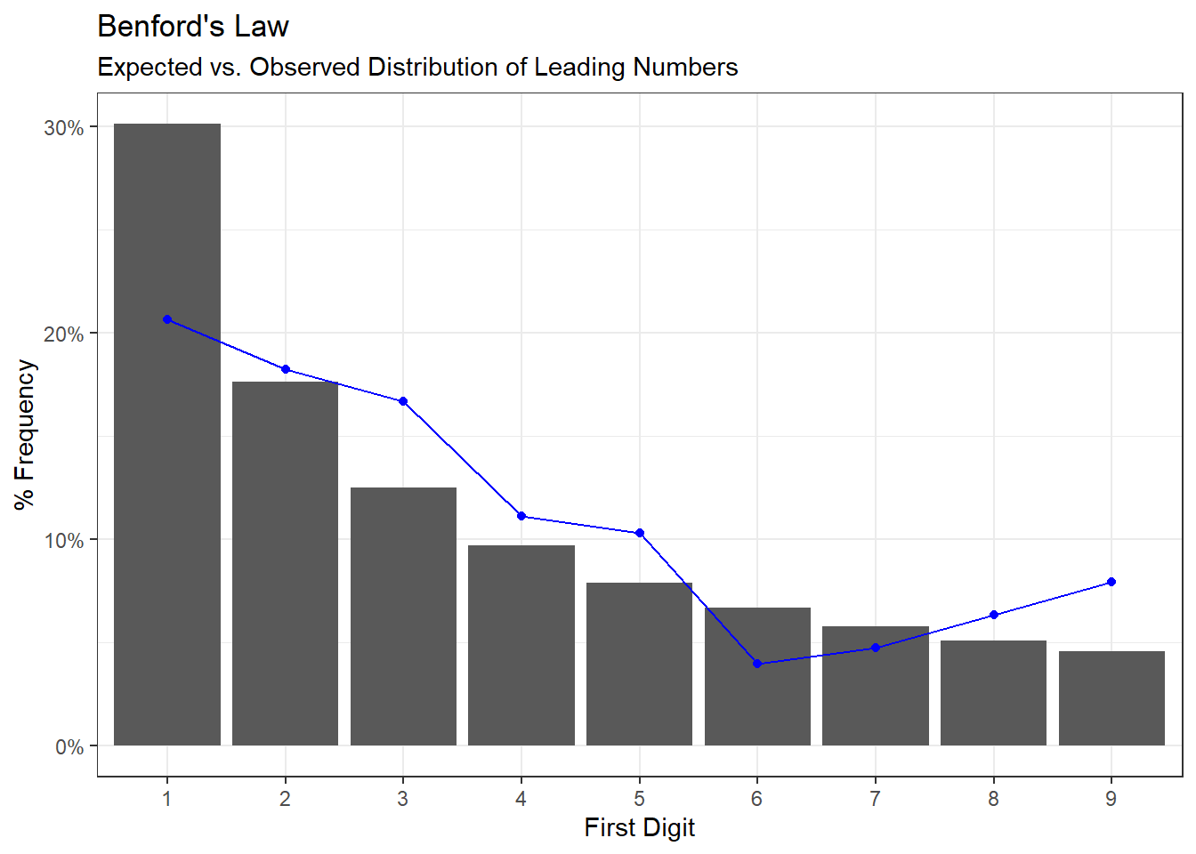
So how do the observed frequencies of campaign spend stack up? There are less 1s and more 9s than you’d expect, but nothing conclusive stands out, especially considering that the observations are on the small side, and that the 40,000 euro limit might have of swayed some things.

Appendix: Fuzzy Joining

Election count data from the electoral commission is in the format Surname Name while data for the spend is in the format Name Surname. Or more concretely:

head(election$candidate)

## [1] "Farrugia Sammy"        "Gauci Tania"           "Buttigieg Anthony"    
## [4] "Abela Ray"             "Apap Meli Sean"        "Attard Joseph Matthew"

head(spend$candidate)

## [1] "Aaron Farrugia"        "Abigail Camilleri"     "Alex Muscat"          
## [4] "Alicia Bugeja Said"    "Alison Zerafa Civelli" "Amanda Spiteri Grech"

We can hack a fast join together using the stringdist and fuzzyjoin packages because the cosine distance between the two names will be similar:

stringdist('Prime Minister', 'Minister Prime', method = 'cosine', q = 2)

## [1] 0.1538462

stringdist('Prime Minister', 'Mister Speaker', method = 'cosine', q = 2)

## [1] 0.5703311

To know whether to join or not, fuzzyjoin needs a Boolean flag, so we can create a wrapper function like so, on a moderately conservative value:

cosine_similarity <- function(left, right) {
  stringdist(left, right, method = "cosine", q = 2) < 0.25
}

and apply it:

result <- fuzzy_left_join(
  election,
  spend,
  by = "candidate",
  match_fun = c("candidate"= cosine_similarity)
)

How well did it do?

## # A tibble: 15 x 2
##    candidate.x           candidate.y          
##    <chr>                 <chr>                
##  1 Farrugia Sammy        <NA>                 
##  2 Gauci Tania           <NA>                 
##  3 Buttigieg Anthony     <NA>                 
##  4 Abela Ray             <NA>                 
##  5 Apap Meli Sean        <NA>                 
##  6 Attard Joseph Matthew Joseph Matthew Attard
##  7 Azzopardi Tanti Keith <NA>                 
##  8 Debattista Deo        Deo Debattista       
##  9 Ellul Andy            Andy Ellul           
## 10 Farrugia Aaron        Aaron Farrugia       
## 11 Galea Cressida        Cressida Galea       
## 12 Grima Chris           <NA>                 
## 13 Herrera Jose'         Jose Herrera         
## 14 Sammut Hili Davina    Davinia Sammut Hili  
## 15 Carabott Darren       Darren Carabott