Electoral Calculus is a well respected UK based political consultancy that has been around for close to 30 years now. Headed by mathematician Martin Baxter, its main interface with the public is to predict UK elections.
“Predicting” elections in the UK, just like the US, is a bit more complicated than polling the national sentiment like those of us in proportional representation countries are used to, since the lower houses of both countries elect members from winner take all districts. This means there can be a huge disparity between the national sentiment and the votes in the districts.
To do this calculation nowadays, Electoral Calculus uses sophisticated regression based techniques like its competitors, but before those methods became available, in a time around 2003-2009, it used a rather different set of models that are probably more similar to what an early Nate Silver used in the late 2000s.
And while advancement is the name of the game, especially in political polling and modelling where papers with tweaks to existing methods seem to be published every other day and new methods coming out every other year, looking back to these older methods is also tremendously educational. I suspect Baxter also shares this historical sentimentality because he’s kept pages on all three of the models we’ll recreate in R on his website.
The plan is to go over:
See how well our STM implementation would have of predicted the 2019 UK General Election
See what an STM says at this point in time
See how an STM on US data compares to 538 congressional forecast
Lastly, it is important to mention that ‘old’ does not mean outdated. The STM is still around in some form, and is working under the hood at Britain Predicts, the collaboration between Britain Elects’s Ben Walker and The New Statesman. Like any other tool, electoral models are more a reflection of their time than anything else. In an era where computation power was low, and data availability sparse, the methods did their best with just a current poll and previous electoral data. The fact that they’re so undemanding is also what lets us code them casually.
Some preparatory work
The House of Commons Library is a great source for both the 2017 and 2019 General Election Results
library(tidyverse)
library(DT)
library(sf)

results_2017 <- read_csv("https://researchbriefings.files.parliament.uk/documents/CBP-7979/HoC-GE2017-constituency-results.csv") %>%
  mutate(con_pct = con/valid_votes*100,
         lab_pct = lab/valid_votes*100,
         lib_pct = ld/valid_votes*100,
         green_pct = green/valid_votes*100,
         snp_pct = snp/valid_votes*100,
         pc_pct = pc/valid_votes*100,
         ref_pct = ukip/valid_votes*100,
         other_pct = (dup+sf+sdlp+uup+alliance+other)/valid_votes*100)

results_2019 <- read_csv("https://researchbriefings.files.parliament.uk/documents/CBP-8749/HoC-GE2019-results-by-constituency-csv.csv") %>%
  mutate(con_pct = con/valid_votes*100,
         lab_pct = lab/valid_votes*100,
         lib_pct = ld/valid_votes*100,
         green_pct = green/valid_votes*100,
         snp_pct = snp/valid_votes*100,
         pc_pct = pc/valid_votes*100,
         ref_pct = brexit/valid_votes*100,
         other_pct = (dup+sf+sdlp+uup+alliance+other)/valid_votes*100)
Uniform National Swing
The simplest ‘model’ is to assume that each of the 650 parliamentary constituencies ‘swung’ by the same amount as the swing between a new poll and the previous election result. This is why discussions of ‘swing’ were (are?) still so popular on BBC while counting.
Coding UNS is easy. We just calculate the swing on a national basis (positive if that party has gained, negative if it has lost) and add it to the previous election results.
For swing, we first work out the 2017 results:
con_nat_pct = sum(results_2017$con)/sum(results_2017$valid_votes) * 100
lab_nat_pct = sum(results_2017$lab)/sum(results_2017$valid_votes) * 100
lib_nat_pct = sum(results_2017$ld)/sum(results_2017$valid_votes) * 100
green_nat_pct = sum(results_2017$green)/sum(results_2017$valid_votes) * 100
snp_nat_pct = sum(results_2017$snp)/sum(results_2017$valid_votes) * 100
pc_nat_pct = sum(results_2017$pc)/sum(results_2017$valid_votes) * 100
ref_nat_pct = sum(results_2017$ukip)/sum(results_2017$valid_votes) * 100
other_nat_pct = sum(results_2017$dup, results_2017$sf, results_2017$sdlp, results_2017$uup, results_2017$alliance, results_2017$other)/sum(results_2017$valid_votes) * 100
For the polls, Wikipedia is surprisingly good for this sort of thing, so I’ll just grab the latest Survation poll from the day before the election.
con_poll = 45
lab_poll = 34
lib_poll = 9
green_poll = 3
snp_poll = 4
pc_poll = 1
other_poll = 3


con_swing = con_poll - con_nat_pct
lab_swing = lab_poll - lab_nat_pct
lib_swing = lib_poll - lib_nat_pct
green_swing = green_poll - green_nat_pct
snp_swing = snp_poll - snp_nat_pct
pc_swing = pc_poll - pc_nat_pct
other_swing = other_poll - other_nat_pct
Then we’ll apply this national swing to all constituencies.
uns_2019 <- results_2017 %>%
  #calculate predicted percentages
  mutate(con_pred = con_pct + con_swing,
         lab_pred = lab_pct + lab_swing,
         lib_pred = lib_pct + lib_swing,
         snp_pred = snp_pct + snp_swing,
         pc_pred = pc_pct + pc_swing,
         green_pred = green_pct + green_swing,
         other_pred = other_pct + other_swing) %>%
  # call seats
  rowwise() %>%
  mutate(seat_call = case_when(
    con_pred > max(lab_pred, lib_pred, green_pred, snp_pred, pc_pred, other_pred) ~ 'CON',
    lab_pred > max(con_pred, lib_pred, green_pred, snp_pred, pc_pred, other_pred) ~ 'LAB',
    lib_pred > max(lab_pred, con_pred, green_pred, snp_pred, pc_pred, other_pred) ~ 'LIB',
    green_pred > max(lab_pred, lib_pred, con_pred, snp_pred, pc_pred, other_pred) ~ 'GRN',
    snp_pred > max(lab_pred, lib_pred, green_pred, con_pred, pc_pred, other_pred) ~ 'SNP',
    pc_pred > max(lab_pred, lib_pred, green_pred, snp_pred, con_pred, other_pred) ~ 'PC',
    TRUE ~ as.character('OTH')))
Which would give us this for 2019:
uns_2019 %>%
  group_by(Party = seat_call) %>%
  tally(name='Seats')%>%
knitr::kable()| Party | Seats |
|---|---|
| CON | 359 |
| GRN | 1 |
| LAB | 216 |
| LIB | 15 |
| OTH | 19 |
| PC | 3 |
| SNP | 37 |
For being so simple, the UNS model works surprisingly well. As it happens, the next evolution, the Transition Model, doesn’t so much address accuracy but a nasty habit of the UNS to either predict negative votes or votes over 100% in some weird seats.
Transition Model
The Transition Model introduces several new ideas, including working out the share of gains each party made nationally, and splitting parties in two, depending on whether they did better or worse since the last election.
If a party did better, the propensity of it’s swing in each seat is calculated, and this proportion of the national vote share is added to the previous election’s result.
If a party did worse, it is assumed to have declined by the same proportion in each seat as in the overall numbers (note, proportion, not percent, so if a party goes down from 45% to 40%, that is a 40/45 = 88% decline, not a -5 swing as in UNS).
My (very ugly) implementation of the transition model as a single R function that takes polls and a dataframe of the previous results
transition_model <- function(
                       con_poll,
                       lab_poll,
                       lib_poll,
                       green_poll,
                       snp_poll,
                       pc_poll,
                       ref_poll,
                       other_poll,
                       dataframe){

  #Applies Electoral Calculus' Transition Model to a UK 650 constituency dataframe.
  #For more info see: https://www.electoralcalculus.co.uk/blogs/newmodel.html#transition


  #work out previous national vote shares automatically
  con_nat_pct = sum(dataframe$con)/sum(dataframe$valid_votes) * 100
  lab_nat_pct = sum(dataframe$lab)/sum(dataframe$valid_votes) * 100
  lib_nat_pct = sum(dataframe$ld)/sum(dataframe$valid_votes) * 100
  green_nat_pct = sum(dataframe$green)/sum(dataframe$valid_votes) * 100
  snp_nat_pct = sum(dataframe$snp)/sum(dataframe$valid_votes) * 100
  pc_nat_pct = sum(dataframe$pc)/sum(dataframe$valid_votes) * 100
  ref_nat_pct = sum(dataframe$ukip)/sum(dataframe$valid_votes) * 100
  other_nat_pct = sum(dataframe$dup, dataframe$sf, dataframe$sdlp, dataframe$uup, dataframe$alliance, dataframe$other)/sum(dataframe$valid_votes) * 100


  #functions we'll use later
  pct_change <- function(prev_election_pct, new_poll_pct){
    return(new_poll_pct/prev_election_pct)
  }

  seat_swing <- function(seat_pct_prev, pct_change){
    return(seat_pct_prev * max(1-pct_change, 0))
  }

  work_out_vote_shares <- function(con_poll, con_nat_pct,
                                   lab_poll, lab_nat_pct,
                                   lib_poll, lib_nat_pct,
                                   green_poll, green_nat_pct,
                                   snp_poll, snp_nat_pct,
                                   pc_poll, pc_nat_pct,
                                   ref_poll, ref_nat_pct,
                                   other_poll, other_nat_pct){

    total_vs <- (max(con_poll - con_nat_pct, 0) + max(lab_poll - lab_nat_pct, 0) + max(lib_poll-lib_nat_pct, 0) + max(green_poll-green_nat_pct, 0) + max(snp_poll-snp_nat_pct, 0) + max(pc_poll-pc_nat_pct, 0) + max(ref_poll-ref_nat_pct, 0) + max(other_poll-other_nat_pct, 0))

    tibble(
      con_vs = max(con_poll - con_nat_pct, 0) / total_vs,
      lab_vs = max(lab_poll - lab_nat_pct, 0) / total_vs,
      lib_vs = max(lib_poll - lib_nat_pct, 0) / total_vs,
      green_vs = max(green_poll - green_nat_pct, 0) /total_vs,
      snp_vs = max(snp_poll - snp_nat_pct, 0) / total_vs,
      pc_vs = max(pc_poll - pc_nat_pct, 0) / total_vs,
      ref_vs = max(ref_poll - ref_nat_pct, 0) / total_vs,
      other_vs = max(other_poll - other_nat_pct, 0) / total_vs)
  }

  ## calculate vote shares
  vs <- work_out_vote_shares(con_poll, con_nat_pct,
                             lab_poll, lab_nat_pct,
                             lib_poll, lib_nat_pct,
                             green_poll, green_nat_pct,
                             snp_poll, snp_nat_pct,
                             pc_poll, pc_nat_pct,
                             ref_poll, ref_nat_pct,
                             other_poll, other_nat_pct)

  ## actual model bit
  transition_model <- dataframe %>%
    #append new polling data
    mutate(con_poll, lab_poll, lib_poll, green_poll, snp_poll, pc_poll, ref_poll, other_poll) %>%
    #append national party voteshare
    bind_cols(vs) %>%
    #calculate seat swing
    mutate(seat_swing =
             (seat_swing(seat_pct_prev = con_pct,
                         pct_change = pct_change(prev_election_pct = con_nat_pct,
                                                 new_poll_pct = con_poll))
              + seat_swing(seat_pct_prev = lab_pct,
                                      pct_change = pct_change(prev_election_pct = lab_nat_pct,
                                                              new_poll_pct = lab_poll))
              + seat_swing(seat_pct_prev = lib_pct,
                           pct_change = pct_change(prev_election_pct = lib_nat_pct,
                                                   new_poll_pct = lib_poll))
              + seat_swing(seat_pct_prev = green_pct,
                           pct_change = pct_change(prev_election_pct = green_nat_pct,
                                                   new_poll_pct = green_poll))
              + seat_swing(seat_pct_prev = snp_pct,
                           pct_change = pct_change(prev_election_pct = snp_nat_pct,
                                                   new_poll_pct = snp_poll))
              + seat_swing(seat_pct_prev = pc_pct,
                           pct_change = pct_change(prev_election_pct = pc_nat_pct,
                                                   new_poll_pct = pc_poll))
              + seat_swing(seat_pct_prev = ref_pct,
                           pct_change = pct_change(prev_election_pct = ref_nat_pct,
                                                   new_poll_pct = ref_poll))
              + seat_swing(seat_pct_prev = other_pct,
                           pct_change = pct_change(prev_election_pct = other_nat_pct,
                                                   new_poll_pct = other_poll))),

           #predict actual votes per party
           con_pred = if_else(con_poll > con_nat_pct,
                              con_pct + (con_vs*seat_swing),
                              (con_pct * con_poll)/con_nat_pct),
           lab_pred = if_else(lab_poll > lab_nat_pct,
                              lab_pct + (lab_vs*seat_swing),
                              (lab_pct * lab_poll)/lab_nat_pct),
           lib_pred = if_else(lib_poll > lib_nat_pct,
                              lib_pct + (lib_vs*seat_swing),
                              (lib_pct * lib_poll)/lib_nat_pct),
           green_pred = if_else(green_poll > green_nat_pct,
                                green_pct + (green_vs*seat_swing),
                                (green_pct * green_poll)/green_nat_pct),
           snp_pred = if_else(snp_poll > snp_nat_pct,
                              snp_pct + (snp_vs*seat_swing),
                              (snp_pct * snp_poll)/snp_nat_pct),
           pc_pred = if_else(pc_poll > pc_nat_pct,
                             pc_pct + (pc_vs*seat_swing),
                             (pc_pct * pc_poll)/pc_nat_pct),
           ref_pred = if_else(ref_poll > ref_nat_pct,
                              ref_pct + (ref_vs*seat_swing),
                              (ref_pct * ref_poll)/ref_nat_pct),
           other_pred = if_else(other_poll > other_nat_pct,
                                other_pct + (other_vs*seat_swing),
                                (other_pct * other_poll)/other_nat_pct)) %>%

    #Name Winning Party
    rowwise() %>%
    mutate(seat_call = case_when(
      con_pred > max(lab_pred, lib_pred, green_pred, snp_pred, pc_pred, ref_pred, other_pred) ~ 'CON',
      lab_pred > max(con_pred, lib_pred, green_pred, snp_pred, pc_pred, ref_pred, other_pred) ~ 'LAB',
      lib_pred > max(lab_pred, con_pred, green_pred, snp_pred, pc_pred, ref_pred, other_pred) ~ 'LIB',
      green_pred > max(lab_pred, lib_pred, con_pred, snp_pred, pc_pred, ref_pred, other_pred) ~ 'GRN',
      snp_pred > max(lab_pred, lib_pred, green_pred, con_pred, pc_pred, ref_pred, other_pred) ~ 'SNP',
      pc_pred > max(lab_pred, lib_pred, green_pred, snp_pred, con_pred, ref_pred, other_pred) ~ 'PC',
      ref_pred > max(lab_pred, lib_pred, green_pred, snp_pred, pc_pred, con_pred, other_pred) ~ 'REF',
      other_pred > max(lab_pred, lib_pred, green_pred, snp_pred, pc_pred, ref_pred, con_pred) ~ 'OTH',
      TRUE ~ as.character(NA)))

  return(transition_model)
}
As for running it:
tm_2019 <- transition_model(con_poll,
                 lab_poll,
                 lib_poll,
                 green_poll,
                 snp_poll,
                 pc_poll,
                 ref_poll = 0,
                 other_poll = 1,
                 results_2017)

tm_2019 %>%
  group_by(Party = seat_call) %>%
  tally(name='Seats') %>%
knitr::kable()| Party | Seats |
|---|---|
| CON | 375 |
| GRN | 2 |
| LAB | 200 |
| LIB | 15 |
| OTH | 18 |
| PC | 3 |
| SNP | 37 |
Strong Transition Model
The Strong Transition Model builds on these ideas a bit further, by splitting each party into two, a ‘strong’ party, with core supporters and a ‘weak’ party with more liquid membership. The ‘weak’ portion of the party is assumed to defect before any member of the ‘strong’ part does.
Once the weak and strong portions of each party are worked nationally, a Transition Model as before is applied to each part.
To start, we’ll define an additional function to calculate the national strong and weak shares of the party. Since EC use a 20% threshold, I’ve set this as the default. Likewise, this takes a previous election result dataframe.
calculate_strong <- function(dataframe, threshold=20){

  #Calculates party shares of 'strong' voters nationally using a weak voter threshold.
  #See: https://www.electoralcalculus.co.uk/blogs/strongmodel.html

strong <- dataframe %>%
  rowwise() %>%
  mutate(con_strong_voters = ((valid_votes + invalid_votes) * max(con_pct-threshold, 0)/100),
         lab_strong_voters = ((valid_votes + invalid_votes) * max(lab_pct-threshold, 0)/100),
         lib_strong_voters = ((valid_votes + invalid_votes) * max(lib_pct-threshold, 0)/100),
         green_strong_voters = ((valid_votes + invalid_votes) * max(green_pct-threshold, 0)/100),
         snp_strong_voters = ((valid_votes + invalid_votes) * max(snp_pct-threshold, 0)/100),
         pc_strong_voters = ((valid_votes + invalid_votes) * max(pc_pct-threshold, 0)/100),
         ref_strong_voters = ((valid_votes + invalid_votes) * max(ref_pct-threshold, 0)/100),
         other_strong_voters = ((valid_votes + invalid_votes) * max(other_pct-threshold, 0)/100),
         total_votes = valid_votes + invalid_votes) %>%
  ungroup() %>%
  summarise(con_strong = sum(con_strong_voters)/sum(total_votes)*100,
            lab_strong = sum(lab_strong_voters)/sum(total_votes)*100,
            lib_strong = sum(lib_strong_voters)/sum(total_votes)*100,
            green_strong = sum(green_strong_voters)/sum(total_votes)*100,
            snp_strong = sum(snp_strong_voters)/sum(total_votes)*100,
            pc_strong = sum(pc_strong_voters)/sum(total_votes)*100,
            ref_strong = sum(ref_strong_voters)/sum(total_votes)*100,
            other_strong = sum(other_strong_voters)/sum(total_votes)*100)

return(strong)
}
Using the 2017 results as an example, these are the shares of ‘strong’ voters for each party:
strong_2017 <- calculate_strong(results_2017)
strong_2017
## # A tibble: 1 x 8
## con_strong lab_strong lib_strong green_strong snp_strong pc_strong ref_strong
## <dbl> <dbl> <dbl> <dbl> <dbl> <dbl> <dbl>
## 1 23.3 21.1 1.08 0.0578 1.39 0.0900 0.000146
## # ... with 1 more variable: other_strong <dbl>And we’ll modify the TM function slightly to do everything in one pop, including taking our newly calculated strong dataframe:
strong_transition_model <-function(
           con_poll,
           lab_poll,
           lib_poll,
           green_poll,
           snp_poll,
           pc_poll,
           ref_poll,
           other_poll,
           dataframe,
           strong_df,
           threshold = 20){

  #Applies Electoral Calculus' Strong Transition Model to a UK 650 constituency dataframe.
  #For more info see: https://www.electoralcalculus.co.uk/blogs/strongmodel.html

  #work out previous national vote shares automatically
  con_nat_pct = strong_df$con_strong
  lab_nat_pct = strong_df$lab_strong
  lib_nat_pct = strong_df$lib_strong
  green_nat_pct = strong_df$green_strong
  snp_nat_pct = strong_df$snp_strong
  pc_nat_pct = strong_df$pc_strong
  ref_nat_pct = strong_df$ref_strong
  other_nat_pct = strong_df$other_strong

  #functions we'll use later
  pct_change <- function(prev_election_pct, new_poll_pct){
    return(new_poll_pct/prev_election_pct)
  }

  seat_swing <- function(seat_pct_prev, pct_change){
    swing <- seat_pct_prev * max(1-pct_change, 0)
    #nan proof this return
    if(is.nan(swing)){
      return(0)
    } else{return(swing)}

  }

  work_out_vote_shares <- function(con_poll, con_nat_pct,
                                   lab_poll, lab_nat_pct,
                                   lib_poll, lib_nat_pct,
                                   green_poll, green_nat_pct,
                                   snp_poll, snp_nat_pct,
                                   pc_poll, pc_nat_pct,
                                   ref_poll, ref_nat_pct,
                                   other_poll, other_nat_pct){

    total_vs <- (max(con_poll - con_nat_pct, 0) + max(lab_poll - lab_nat_pct, 0) + max(lib_poll-lib_nat_pct, 0) + max(green_poll-green_nat_pct, 0) + max(snp_poll-snp_nat_pct, 0) + max(pc_poll-pc_nat_pct, 0) + max(ref_poll-ref_nat_pct, 0) + max(other_poll-other_nat_pct, 0))

    tibble(
      con_vs = max(con_poll - con_nat_pct, 0) / total_vs,
      lab_vs = max(lab_poll - lab_nat_pct, 0) / total_vs,
      lib_vs = max(lib_poll - lib_nat_pct, 0) / total_vs,
      green_vs = max(green_poll - green_nat_pct, 0) / total_vs,
      snp_vs = max(snp_poll - snp_nat_pct, 0) / total_vs,
      pc_vs = max(pc_poll - pc_nat_pct, 0) / total_vs,
      ref_vs = max(ref_poll - ref_nat_pct, 0) / total_vs,
      other_vs = max(other_poll - other_nat_pct, 0) / total_vs)
  }

  vs <- work_out_vote_shares(con_poll, con_nat_pct,
                             lab_poll, lab_nat_pct,
                             lib_poll, lib_nat_pct,
                             green_poll, green_nat_pct,
                             snp_poll, snp_nat_pct,
                             pc_poll, pc_nat_pct,
                             ref_poll, ref_nat_pct,
                             other_poll, other_nat_pct)


  transition_model <- dataframe %>%

    #append new polling data
    mutate(con_poll, lab_poll, lib_poll, green_poll, snp_poll, pc_poll, ref_poll, other_poll) %>%
    #append national party voteshare
    bind_cols(vs) %>%
    rowwise() %>%
    #calculate seat swing
    mutate(
      seat_swing = (seat_swing(seat_pct_prev = max(con_pct-threshold, 0),
                               pct_change = pct_change(prev_election_pct = con_nat_pct,
                                                       new_poll_pct = con_poll))
                    + seat_swing(seat_pct_prev = max(lab_pct-threshold, 0),
                                 pct_change = pct_change(prev_election_pct = lab_nat_pct,
                                                         new_poll_pct = lab_poll))
                    + seat_swing(seat_pct_prev = max(lib_pct-threshold, 0),
                                 pct_change = pct_change(prev_election_pct = lib_nat_pct,
                                                         new_poll_pct = lib_poll))
                    + seat_swing(seat_pct_prev = max(green_pct-threshold, 0),
                                 pct_change = pct_change(prev_election_pct = green_nat_pct,
                                                         new_poll_pct = green_poll))
                    + seat_swing(seat_pct_prev = max(snp_pct-threshold, 0),
                                 pct_change = pct_change(prev_election_pct = snp_nat_pct,
                                                         new_poll_pct = snp_poll))
                    + seat_swing(seat_pct_prev = max(pc_pct-threshold, 0),
                                 pct_change = pct_change(prev_election_pct = pc_nat_pct,
                                                         new_poll_pct = pc_poll))
                    + seat_swing(seat_pct_prev = max(ref_pct-threshold, 0),
                                 pct_change = pct_change(prev_election_pct = ref_nat_pct,
                                                         new_poll_pct = ref_poll))
                    + seat_swing(seat_pct_prev = max(other_pct-threshold, 0),
                                 pct_change = pct_change(prev_election_pct = other_nat_pct,
                                                         new_poll_pct = other_poll))),

           #predict strong actual votes per party
           con_pred_s = if_else(con_poll > con_nat_pct,
                                max(con_pct-threshold, 0) + (con_vs*seat_swing),
                                (max(con_pct-threshold, 0) * con_poll)/con_nat_pct),
           lab_pred_s = if_else(lab_poll > lab_nat_pct,
                                max(lab_pct-threshold, 0) + (lab_vs*seat_swing),
                                (max(lab_pct-threshold, 0) * lab_poll)/lab_nat_pct),
           lib_pred_s = if_else(lib_poll > lib_nat_pct,
                                max(lib_pct-threshold, 0) + (lib_vs*seat_swing),
                                (max(lib_pct-threshold, 0) * lib_poll)/lib_nat_pct),
           green_pred_s = if_else(green_poll > green_nat_pct,
                                  max(green_pct-threshold, 0) + (green_vs*seat_swing),
                                  (max(green_pct-threshold, 0) * green_poll)/green_nat_pct),
           snp_pred_s = if_else(snp_poll > snp_nat_pct,
                                max(snp_pct-threshold, 0) + (snp_vs*seat_swing),
                                (max(snp_pct-threshold, 0) * snp_poll)/snp_nat_pct),
           pc_pred_s = if_else(pc_poll > pc_nat_pct,
                               max(pc_pct-threshold, 0) + (pc_vs*seat_swing),
                               (max(pc_pct-threshold, 0) * pc_poll)/pc_nat_pct),
           ref_pred_s = if_else(ref_poll > ref_nat_pct,
                                max(ref_pct-threshold, 0) + (ref_vs*seat_swing),
                                (max(ref_pct-threshold, 0) * ref_poll)/ref_nat_pct),
           other_pred_s = if_else(other_poll > other_nat_pct,
                                  max(other_pct-threshold, 0) + (other_vs*seat_swing),
                                  (max(other_pct-threshold, 0) * other_poll)/other_nat_pct),

      #predict weak actual votes per party
           con_pred_w = if_else(con_poll > con_nat_pct,
                                con_pct-con_pred_s + (con_vs*seat_swing),
                                ((con_pct-con_pred_s) * con_poll)/con_nat_pct),
           lab_pred_w = if_else(lab_poll > lab_nat_pct,
                                lab_pct-lab_pred_s + (lab_vs*seat_swing),
                                ((lab_pct-lab_pred_s) * lab_poll)/lab_nat_pct),
           lib_pred_w = if_else(lib_poll > lib_nat_pct,
                                lib_pct-lib_pred_s + (lib_vs*seat_swing),
                                ((lib_pct-lib_pred_s) * lib_poll)/lib_nat_pct),
           green_pred_w = if_else(green_poll > green_nat_pct,
                                  green_pct-green_pred_s + (green_vs*seat_swing),
                                  ((green_pct-green_pred_s) * green_poll)/green_nat_pct),
           snp_pred_w = if_else(snp_poll > snp_nat_pct,
                                snp_pct-snp_pred_s + (snp_vs*seat_swing),
                                ((snp_pct-snp_pred_s) * snp_poll)/snp_nat_pct),
           pc_pred_w = if_else(pc_poll > pc_nat_pct,
                               pc_pct-pc_pred_s + (pc_vs*seat_swing),
                               ((pc_pct-pc_pred_s) * pc_poll)/pc_nat_pct),
           ref_pred_w = if_else(ref_poll > ref_nat_pct,
                                ref_pct-ref_pred_s + (ref_vs*seat_swing),
                                ((ref_pct-ref_pred_s) * ref_poll)/ref_nat_pct),
           other_pred_w = if_else(other_poll > other_nat_pct,
                                  other_pct-other_pred_s + (other_vs*seat_swing),
                                  ((other_pct-other_pred_s) * other_poll)/other_nat_pct),

           #final tally
           con_pred = if_else(is.nan(con_pred_s+con_pred_w),
                              0,
                              con_pred_s+con_pred_w),
           lab_pred = if_else(is.nan(lab_pred_s+lab_pred_w),
                              0,
                              lab_pred_s+lab_pred_w),
           lib_pred = if_else(is.nan(lib_pred_s+lib_pred_w),
                              0,
                              lib_pred_s+lib_pred_w),
           green_pred = if_else(is.nan(green_pred_s+green_pred_w),
                                0,
                                green_pred_s+green_pred_w),
           snp_pred = if_else(is.nan(snp_pred_s+snp_pred_w),
                              0,
                              snp_pred_s+snp_pred_w),
           pc_pred = if_else(is.nan(pc_pred_s+pc_pred_w),
                             0,
                             pc_pred_s+pc_pred_w),
           ref_pred = if_else(is.nan(ref_pred_s+ref_pred_w),
                              0,
                              ref_pred_s+ref_pred_w),
           other_pred = if_else(is.nan(other_pred_s+other_pred_w),
                                0,
                                other_pred_s+other_pred_w)) %>%
    #Seat call
    mutate(
      seat_call = case_when(
        con_pred > max(lab_pred, lib_pred, green_pred, snp_pred, pc_pred, ref_pred, other_pred) ~ 'CON',
        lab_pred > max(con_pred, lib_pred, green_pred, snp_pred, pc_pred, ref_pred, other_pred) ~ 'LAB',
        lib_pred > max(lab_pred, con_pred, green_pred, snp_pred, pc_pred, ref_pred, other_pred) ~ 'LIB',
        green_pred > max(lab_pred, lib_pred, con_pred, snp_pred, pc_pred, ref_pred, other_pred) ~ 'GRN',
        snp_pred > max(lab_pred, lib_pred, green_pred, con_pred, pc_pred, ref_pred, other_pred) ~ 'SNP',
        pc_pred > max(lab_pred, lib_pred, green_pred, snp_pred, con_pred, ref_pred, other_pred) ~ 'PC',
        ref_pred > max(lab_pred, lib_pred, green_pred, snp_pred, pc_pred, con_pred, other_pred) ~ 'REF',
        other_pred > max(lab_pred, lib_pred, green_pred, snp_pred, pc_pred, ref_pred, con_pred) ~ 'OTH',
        TRUE ~ as.character(NA)))


  return(transition_model)
  }
As for running it:
stm_2019 <- strong_transition_model(con_poll = con_poll - strong_2017$con_strong,
                             lab_poll = lab_poll - strong_2017$lab_strong,
                             lib_poll = lib_poll - strong_2017$lib_strong,
                             green_poll = green_poll - strong_2017$green_strong,
                             snp_poll = snp_poll - strong_2017$snp_strong,
                             pc_poll = pc_poll - strong_2017$pc_strong,
                             ref_poll = 0,
                             other_poll = 3 - strong_2017$other_strong,
                             dataframe = results_2017,
                             strong_df = strong_2017)

stm_2019 %>%
  group_by(Party = seat_call) %>%
  tally(name='Seats')%>%
knitr::kable()| Party | Seats |
|---|---|
| CON | 364 |
| GRN | 1 |
| LAB | 204 |
| LIB | 17 |
| OTH | 19 |
| PC | 4 |
| SNP | 41 |
How Well did we Predict 2019?
Let’s see how the three models compare. I’ll pluck some relevant columns from all the dataframes, and join them to the 2019 actual results.
interesting_columns <- c('ons_id', 'seat_call', 'con_pred', 'lab_pred', 'lib_pred')

west_hex_map <- parlitools::west_hex_map

#Data for map
pred_data <- west_hex_map %>%

  #join UNS preds
  left_join(uns_2019 %>%
    select(all_of(interesting_columns))%>%
    rename_all(list(~paste0('uns_', .))),
      by = c("gss_code" = "uns_ons_id")) %>%

  #Join TM preds
  left_join(tm_2019 %>%
    select(all_of(interesting_columns)) %>%
    rename_all(list(~paste0('tm_', .))),
      by = c("gss_code" = "tm_ons_id")) %>%

  #Join STM preds
  left_join(stm_2019 %>%
    select(all_of(interesting_columns)) %>%
    rename_all(list(~paste0('stm_', .))),
      by = c("gss_code" = "stm_ons_id")) %>%

  #Join actual 2019 results
  left_join(results_2019 %>%
              select(c('ons_id', 'first_party', 'con_pct', 'lab_pct', 'lib_pct')),
                by = c('gss_code' = 'ons_id')) %>%
  mutate(first_party = toupper(first_party),
         first_party = case_when(first_party %in% c('CON', 'LAB', 'SNP', 'PC') ~ first_party,
                                 first_party == 'GREEN' ~ 'GRN',
                                 first_party == 'LD' ~ 'LIB',
                                 TRUE ~ 'OTH'))
A cartogram is always easier for these sort of visualisations, and the parlitools package by Evan Odell has some great functionality to make this easier.
The constituencies we got right I kept grey, the ones we predicted wrong are:
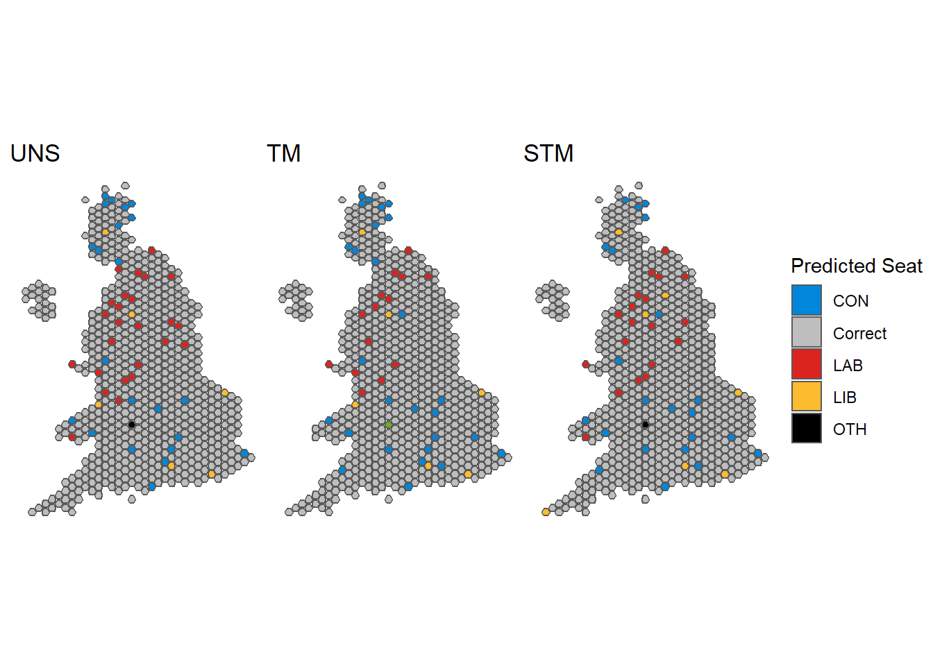
Our STM got 601 constituencies right and 49 wrong. Part of the problem is in Scotland, where the Great Britain wide poll we fitted significantly diluted SNP support, so the Conservatives end up getting a few SNP seats.
Another way to visualize it is by plotting predicted vs actual voteshares in each of the 650 constituencies. It becomes readily apparent that STM for some reason overestimated the Lib Dems.
ggplot(pred_data)+
  geom_point(aes(x=stm_con_pred, y = con_pct), color = '#0087DC', alpha = 0.5)+
  geom_point(aes(x=stm_lab_pred, y = lab_pct), color = '#DC241F', alpha = 0.5)+
  geom_point(aes(x=stm_lib_pred, y = lib_pct), color = '#FDBB30', alpha = 0.5)+
  xlab('STM Predictions')+
  ylab('Actual Results')+
  geom_abline()+
  theme_bw()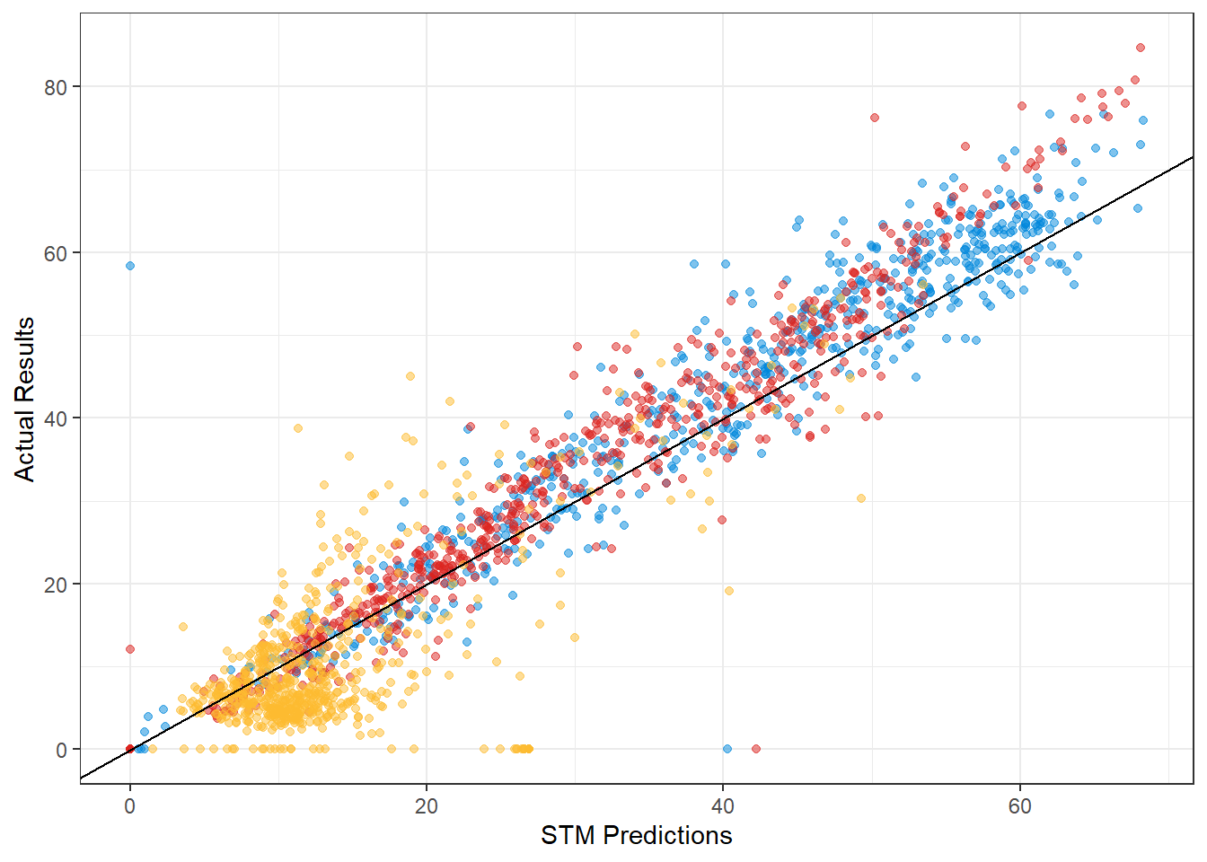
Predicting Now
And how does it look if we run an STM using the most current polling data? For ‘current’, I’ll use this YouGov poll from a week ago at time of writing.
I’ll also bump the threshold up to 25%, because according to the methodology write up, New Statesman uses a much higher weak voter threshold based on British Election Study figures that show that nearly a third of Britons consider voting for a different party.
strong_2019 <- calculate_strong(results_2019, threshold = 25)

stm_now <- strong_transition_model(con_poll = 32 - strong_2019$con_strong,
                             lab_poll = 39 - strong_2019$lab_strong,
                             lib_poll = 12 - strong_2019$lib_strong,
                             green_poll = 8 - strong_2019$green_strong,
                             snp_poll = 4 - strong_2019$snp_strong,
                             pc_poll = 1 - strong_2019$pc_strong,
                             ref_poll = 0,
                             other_poll = 3 - strong_2019$other_strong,
                             dataframe = results_2019,
                             strong_df = strong_2019)

stm_now %>%
  group_by(Party = seat_call) %>%
  tally(name='Seats') %>%
knitr::kable()| Party | Seats |
|---|---|
| CON | 222 |
| GRN | 1 |
| LAB | 316 |
| LIB | 34 |
| OTH | 19 |
| PC | 4 |
| SNP | 54 |
The results are fairly close to Britan Predicts’, but ours understate Labour, overstate Conservative and Lib Dems a tad.
Plotted as a map:
uk_map %>%
  left_join(stm_now, by = c("PCON19CD" = "ons_id")) %>%
  ggplot(aes(fill = seat_call))+
  geom_sf()+
  coord_sf()+
  scale_fill_manual(values = c("#0087DC", "#6AB023",
                    "#DC241F", "#FDBB30", "#DDDDDD",
                    '#008142', '#FFFF00'),
                   name= "Predicted Seat")+
  theme_bw()+
  labs(title = '')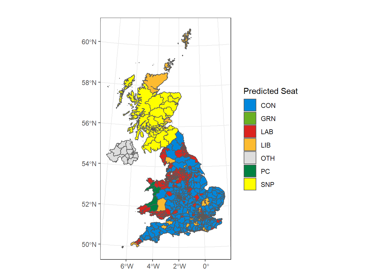
Or as an interactive cartogram, based on this vignette (you can mouse over and zoom in):
The 30 constituencies with the largest projected Conservative losses are:
library(ggtext)
library(ggalt)

stm_now %>%
  mutate(first_party = toupper(first_party),
         first_party = case_when(first_party %in% c('CON', 'LAB', 'SNP', 'PC') ~ first_party,
                                 first_party == 'GREEN' ~ 'GRN',
                                 first_party == 'LD' ~ 'LIB',
                                 TRUE ~ 'OTH')) %>%
  filter(first_party != seat_call) %>%
  select(constituency_name, con_pct, con_pred) %>%
  mutate(diff = con_pred-con_pct) %>%
  arrange(diff) %>%
  head(25) %>%
  ggplot(aes(x=con_pct,
             xend=con_pred,
             y=fct_reorder(constituency_name, -con_pct),
             group=constituency_name))+
  geom_dumbbell(color="#0087DC",
                      size=0.75,
                      colour_xend ="black")+
  theme_bw()+
  ylab('')+
  xlab('Conservative % of vote')+
  labs(title = 'Constituencies with largest predicted Conservative losses',
       subtitle = "Predicted Result vs. <span style='color: #0087DC;'>Previous Election Result<span>")+
  theme(plot.subtitle = element_markdown(face="bold"))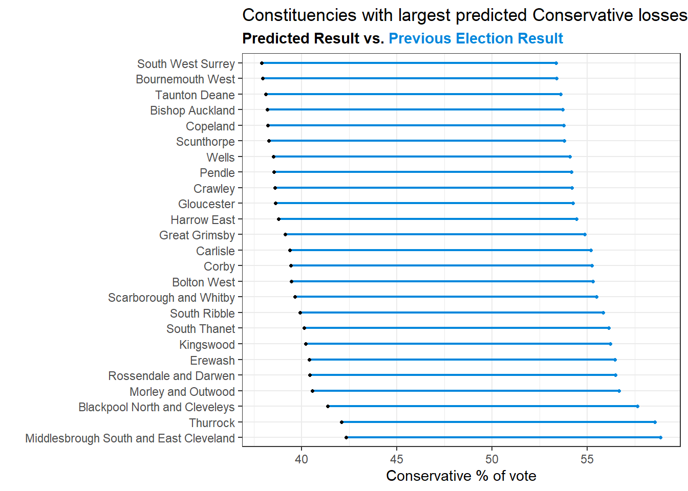
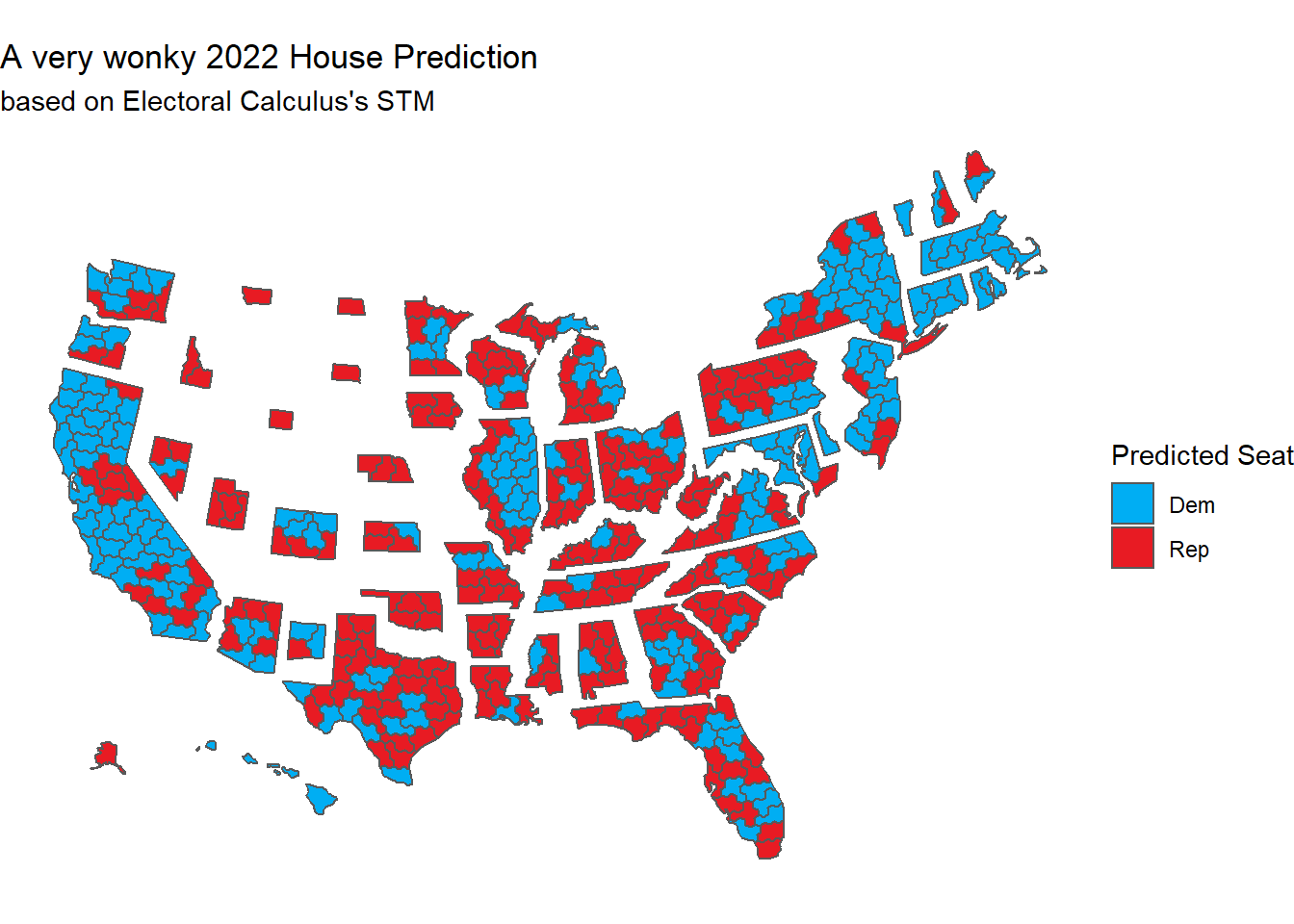
Running an STM for the 2022 US House Elections
This is more fun than anything, but how sensible would an STM result be for the US House? Since the underlying mechanics are the same, it’s not unreasonable to assume that it might work well. To do this, I used the U.S. House 1976–2020 published by the MIT Election Data and Science Lab here to get the 2022 result. The wrangling is just to create a roughly equivalent dataframe to the UK one:
##Wrangle with house data
us_house <- read_csv(path) %>%
  filter(year==2020) %>%
  #flatten one row per seat
  group_by(state_po, district) %>%
  summarise(
    dem_pct = max(if_else(party == 'DEMOCRAT', candidatevotes/totalvotes, 0),
                          na.rm=T)*100,
    rep_pct = max(if_else(party == 'REPUBLICAN', candidatevotes/totalvotes, 0),
                          na.rm=T)*100,
    other_pct = max(if_else(!party %in% c('REPUBLICAN', 'DEMOCRAT'), candidatevotes/totalvotes, 0), na.rm=T)*100,
    total_votes = max(totalvotes))%>%
  mutate(district = as.numeric(district))

head(us_house)
## # A tibble: 6 x 6
## # Groups: state_po [2]
## state_po district dem_pct rep_pct other_pct total_votes
## <chr> <dbl> <dbl> <dbl> <dbl> <dbl>
## 1 AK 0 45.3 54.4 0.335 353165
## 2 AL 1 35.5 64.4 0.0915 329075
## 3 AL 2 34.7 65.2 0.0945 303569
## 4 AL 3 32.5 67.5 0.0791 322234
## 5 AL 4 17.7 82.2 0.0752 318029
## 6 AL 5 0 95.8 4.19 264160After that I just modified both functions slightly and plugged in the latest numbers from 538’s generic ballot tracker. My intuition tells me that US politics is a great deal more polarised at the moment, so I bumped the weak voter threshold back to 20% (lower propensity to switch parties).
threshold=20
strong <- us_house %>%
  rowwise() %>%
  mutate(dem_strong_voters = total_votes * max(dem_pct-threshold, 0)/100,
         rep_strong_voters = total_votes * max(rep_pct-threshold, 0)/100,
         other_strong_voters = total_votes * max(other_pct-threshold, 0)/100) %>%
  ungroup() %>%
  summarise(dem_strong = sum(dem_strong_voters)/sum(total_votes)*100,
            rep_strong = sum(rep_strong_voters)/sum(total_votes)*100,
            other_strong = sum(other_strong_voters)/sum(total_votes)*100)


us <- us_strong_transition_model(dem_poll = 43.9 - strong$dem_strong,
                             rep_poll = 44.1- strong$rep_strong,
                             other_poll = 0,
                             dataframe = us_house,
                             strong_df = strong)

us %>%
  group_by(Party = seat_call) %>%
  tally(name='Seats')
## # A tibble: 2 x 2
## Party Seats
## <chr> <int>
## 1 Dem 196
## 2 Rep 240The latest prediction from 538 is 202/233, so we’re off by roughly 7 seats. As for mapping it, Shiro Kuriwaki posted a great sf/ggplot implementation of Daily Kos’ cartogram, specifically the variety published by Daniel Donner:
library(donnermap)
library(ggthemes)

cd_shp %>%
  mutate(CDLABEL = as.numeric(CDLABEL),
         CDLABEL = if_else(is.na(CDLABEL), 0, CDLABEL)) %>%
  left_join(us, by = c('STATEAB' = 'state_po',
                       'CDLABEL' = 'district')) %>%
  ggplot(aes(fill = seat_call))+
  geom_sf()+
  coord_sf()+
  theme_void()+
  scale_fill_manual(values = c("#00aef3","#E81B23"),
                   name= "Predicted Seat")+
  labs(title = 'A very wonky 2022 House Prediction',
       subtitle = "based on Electoral Calculus's STM")