Frasier is my favourite TV show of all time. I’ve watched the entire series many times over from start to finish. So when I found a dataset on kaggle with both episode meta-information and the scripts, I knew I had to do a write up on it.
Who has the most words?
Frasier is predominantly a character oriented show: nothing very exciting or spectacular happens in terms of plot, and when it does, the emphasis is on how the characters handle and react to often absurd situations. So one way to get a basic idea of what the show is about is to see who has the most air time.
To do this I’ll use the usual tidytext unnest_tokens() workflow mentioned in other blogposts, so I won’t delve too much in it:
CharactersbyWords <- script %>%
  unnest_tokens(words, dialog) %>%
  group_by(cast) %>%
  summarise(totalwords = n()) %>%
  top_n(15) %>%
  ggplot(aes(fct_reorder(cast, totalwords), totalwords, fill = cast))+
  geom_col()+
  coord_flip()+
  scale_y_continuous(label = comma)+
  xlab("")+
  ylab("Total Words in Entire Show")+
  theme(legend.position = "none")
## Selecting by totalwordsCharactersbyWords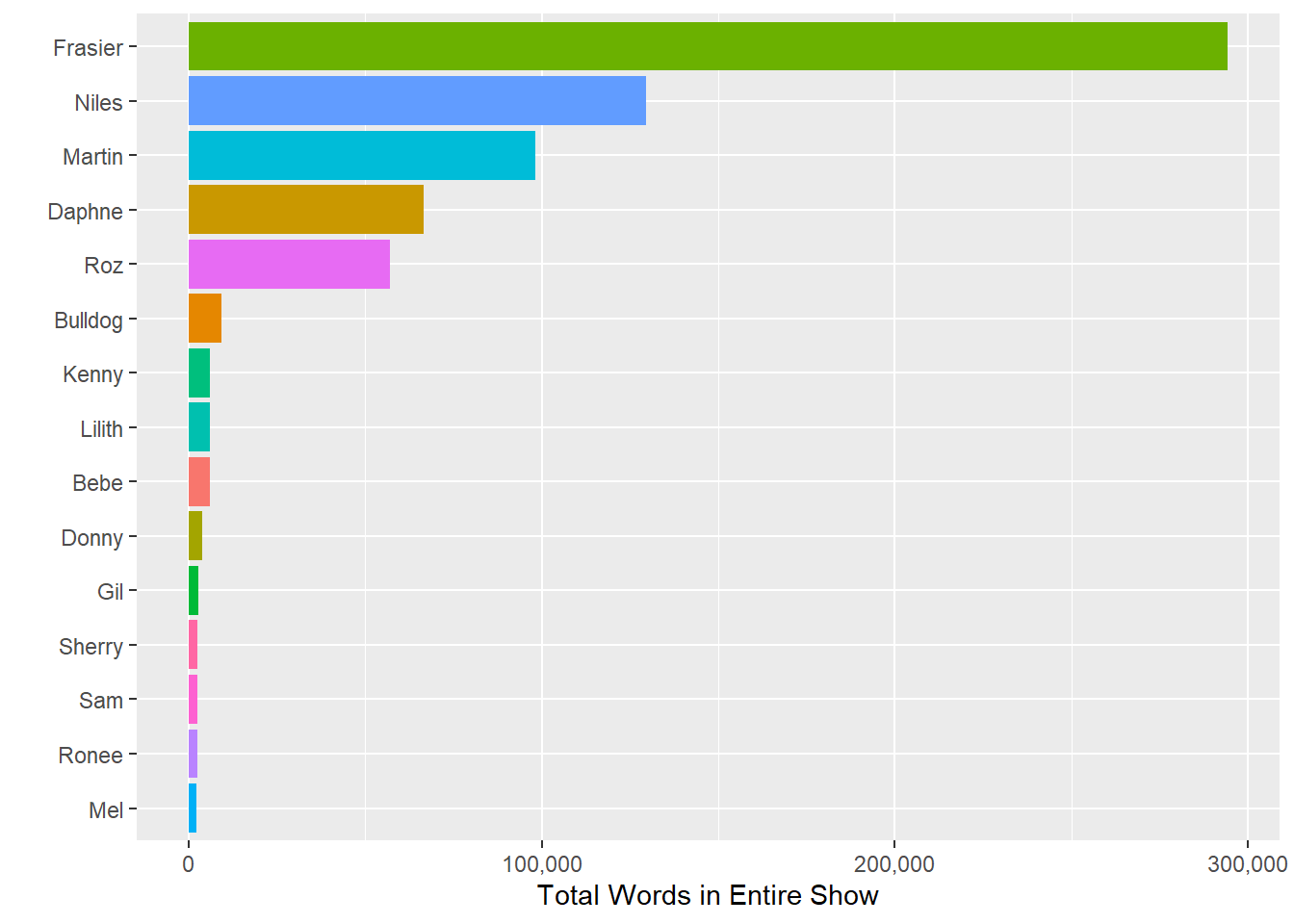
And predictably, the titular character gets most of the word count, nearly double that of the second place character, Niles.
TF-IDF: What are those words?
While a raw count can tell us how many words came out of each character, TF-IDF can tell us which words are more likely to come from one character as opposed to the other.
##TF-IDF
unnested_dialogue_words <- ScriptCleaned %>%
  unnest_tokens(word, dialog) %>%
  filter(!is.na(word)) %>%
  anti_join(stop_words) %>%
  count(cast, word, sort = TRUE)
## Joining, by = "word"total_words <- ScriptCleaned %>%
group_by(cast) %>%
summarize(total = sum(n()))
dialogue_words <- left_join(unnested_dialogue_words, total_words) ## Joining, by = "cast"dialogue_words <- dialogue_words %>%
filter(n > 30) %>%
bind_tf_idf(word, cast, n) %>%
arrange(desc(tf_idf))
plot_tf_idf <- dialogue_words %>%
filter(cast %in% c("Niles", "Frasier", "Roz", "Gil", "Martin", "Daphne", "Bebe", "Lillith", "Kenny", "Bulldog", "Freddie")) %>%
group_by(cast) %>%
top_n(10, tf_idf) %>%
ungroup() %>%
mutate(word = reorder(word, tf_idf)) %>%
ggplot(aes(word, tf_idf, fill = cast)) +
geom_col(show.legend = FALSE) +
labs(x = NULL, y = "TF-IDF Score", title = "Top 10 TF-IDF Terms") +
facet_wrap(~cast, ncol = 3, scales = "free") +
coord_flip()
plot_tf_idf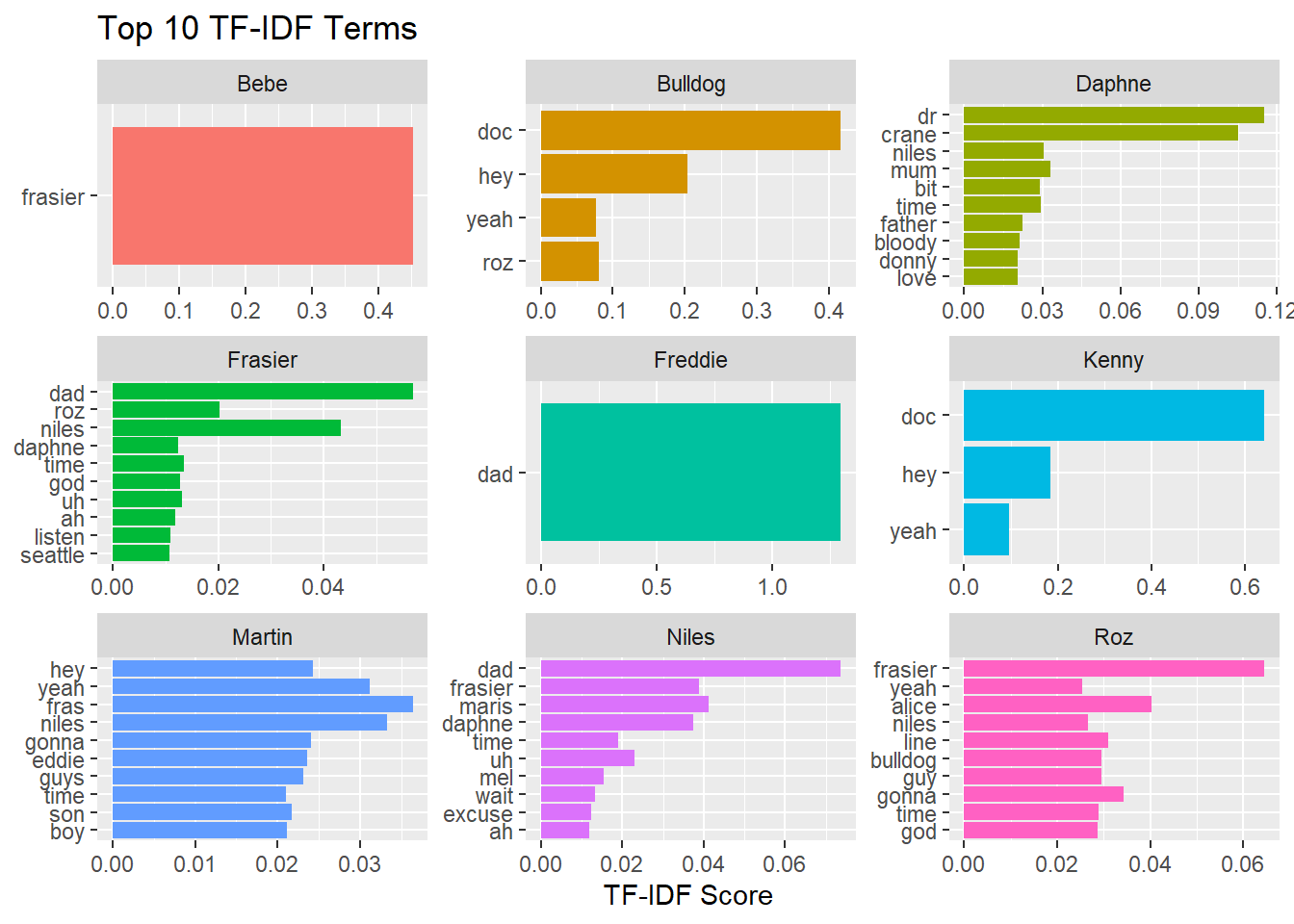
The results make sense: Bebe, Frasier’s agent, mostly appears speaking to Frasier. So does Freddie, Frasier’s son, who is much more likely to use “dad”. Bulldog and Kenny, Frasier’s coworkers, often greet him with “Hey Doc”, while Daphne is much more likely to opt for “Dr. Crane”, and being from Manchester, more predisposed to use “bloody”.
Frasier’s trademark radio greeting “I’m Listening Seattle” probably explains his last two tf-idf terms, and Martin is often talking to his sons/boys or his dog Eddie.
Niles is also much more likely to mention his two ex-wives Maris and Mel and Roz her daughter Alice.
Sentiment through the show
Since we had the scripts I thought it would be interesting to compute how much sentiment varies across the episodes.
It turns out that across the episodes, the variation might be sizeable, but every season seems to have a consistent mean.
SentimentAnalysis <- script %>%
  mutate(dialog = str_replace(dialog, " *\\[.*?\\] *", "")) %>%
  unnest_tokens(word, dialog) %>%
  inner_join(get_sentiments("afinn")) %>%
  left_join(episode) %>%
  select(c("season", "episode", "cast", "word", "value", "Aired_date", "url")) %>%
  group_by(season, episode) %>%
  summarise(episode_sentiment = mean(value))
## Joining, by = "word"## Joining, by = "url"## `summarise()` has grouped output by 'season'. You can override using the `.groups` argument.ggplot(SentimentAnalysis, aes(episode, episode_sentiment, col = factor(season)))+
geom_point()+
geom_smooth(method = "lm", se = F)+
facet_wrap(~season)+
theme(legend.position = "none")## `geom_smooth()` using formula 'y ~ x'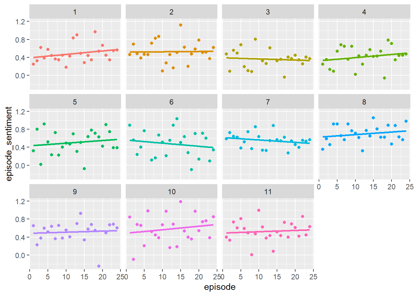
This might make sense in terms of arcs within the season. You’d want to generate a mix of emotions in your viewers to make sure they keep tuning in.
Words per episode
And since we have the unnested script handy, we can see the distribution of words per episode:
## Joining, by = "url"## `summarise()` has grouped output by 'season'. You can override using the `.groups` argument.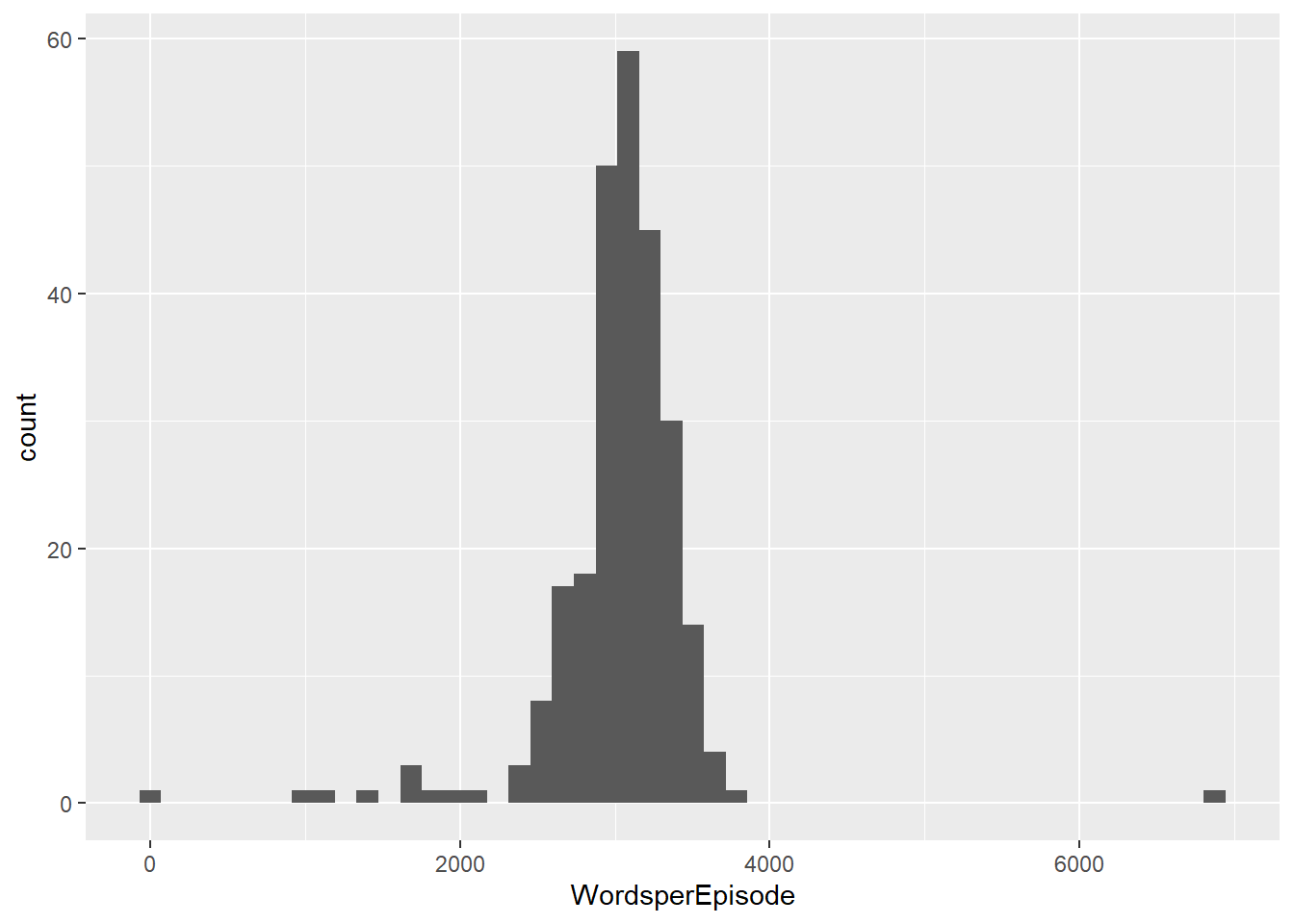
Turns out that the mean words per episode are 3,024.
Maris
Maris is probably one of the greatest running gags in all of television. She first appeared in the show as Niles’ insanely rich wife (we later learn, thanks to her family’s urinal cake business). Though at first she probably was uncast as a way to save some money for a new show, producers later said that even if they wanted to cast her, they couldn’t possibly find an actress to fit to the outlandish caricature the writers had devised. So for 11 seasons she goes unseen.
Using Stringr’s str_detect() function, we could easily check whether Maris appeared in an episode or not.
##Maris?

Maris <- episode %>%
  select(url, season, episode) %>%
  left_join(script) %>%
  mutate(has_maris = str_detect(dialog, c("Maris", "maris"))) %>%
  group_by(season, episode) %>%
  summarise(CountMaris = sum(has_maris, na.rm = T)) %>%
  mutate(HasMaris = if_else(CountMaris > 0, "Yes", "No", "No"))
## Joining, by = "url"## `summarise()` has grouped output by 'season'. You can override using the `.groups` argument.ggplot(Maris, aes(x=episode, y = HasMaris, col = HasMaris))+
geom_point()+
facet_wrap(~season)+
xlab("Episode")+
ylab("Is Maris Mentioned?")+
theme(legend.position = "none")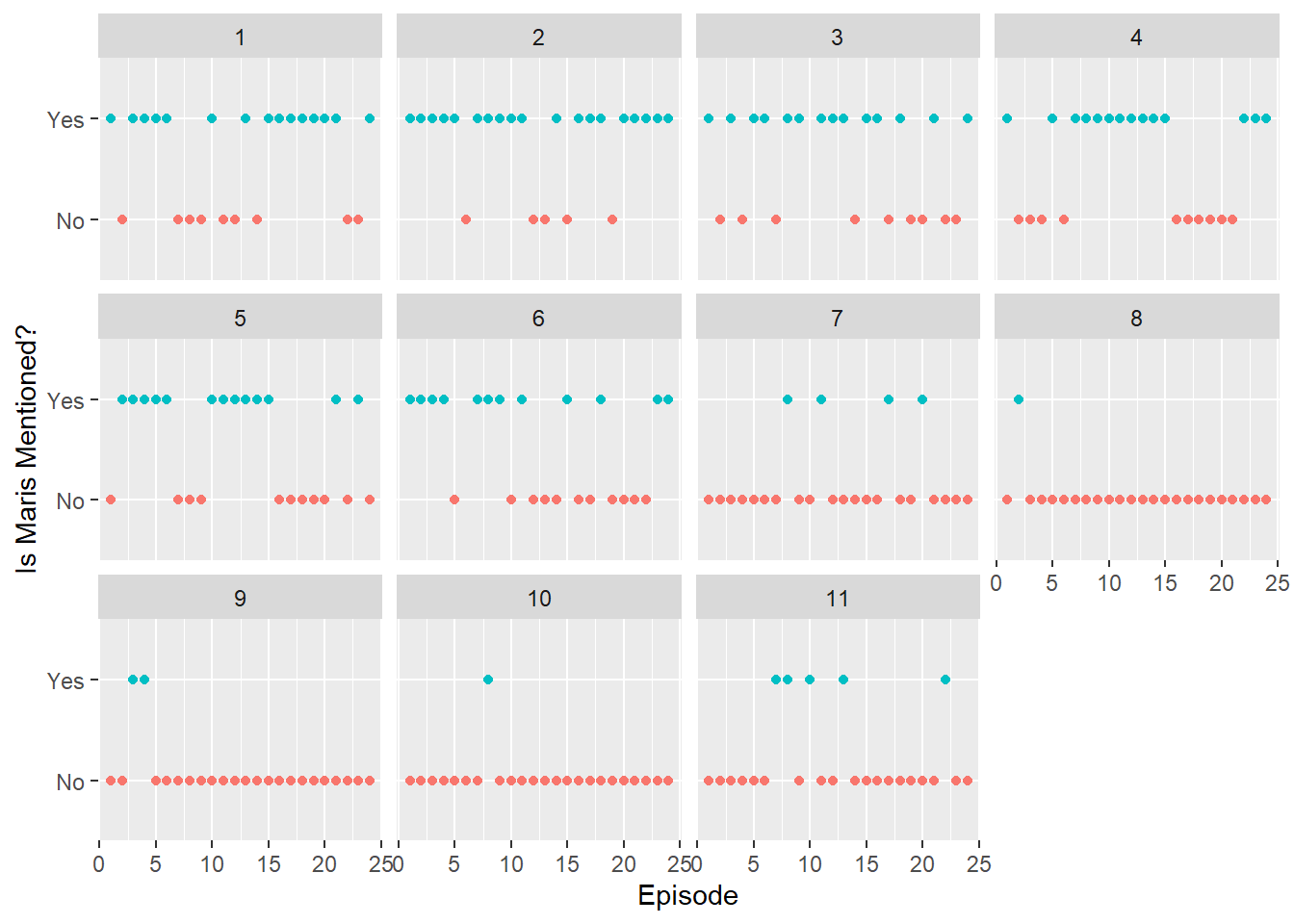
From the looks of things, she featured pretty heavily in the first 6 seasons, then diminishing, before making a few final appearances in season 11 to end her chapter within the show.
Did lines per Character change across the seasons?
This is a more sophisticated version of the very first graph I plotted in this post. Rather than counting all the words, it counts all the lines in each episode per character. By plotting this over the seasons, we can see if some characters became more important or less important than others.
LinesPerEpisode <- script %>%
  group_by(url) %>%
  count(cast, sort = T) %>%
  left_join(episode) %>%
  select(season, episode, cast, n) %>%
  filter(cast %in% c("Frasier", "Niles", "Martin",
                     "Daphne", "Roz"))
## Joining, by = "url"## Adding missing grouping variables: `url`ggplot(LinesPerEpisode, aes(x = episode, y = n, color = cast))+
geom_point(alpha = 0.5)+
geom_smooth(se=F)+
facet_wrap(~season)## `geom_smooth()` using method = 'loess' and formula 'y ~ x'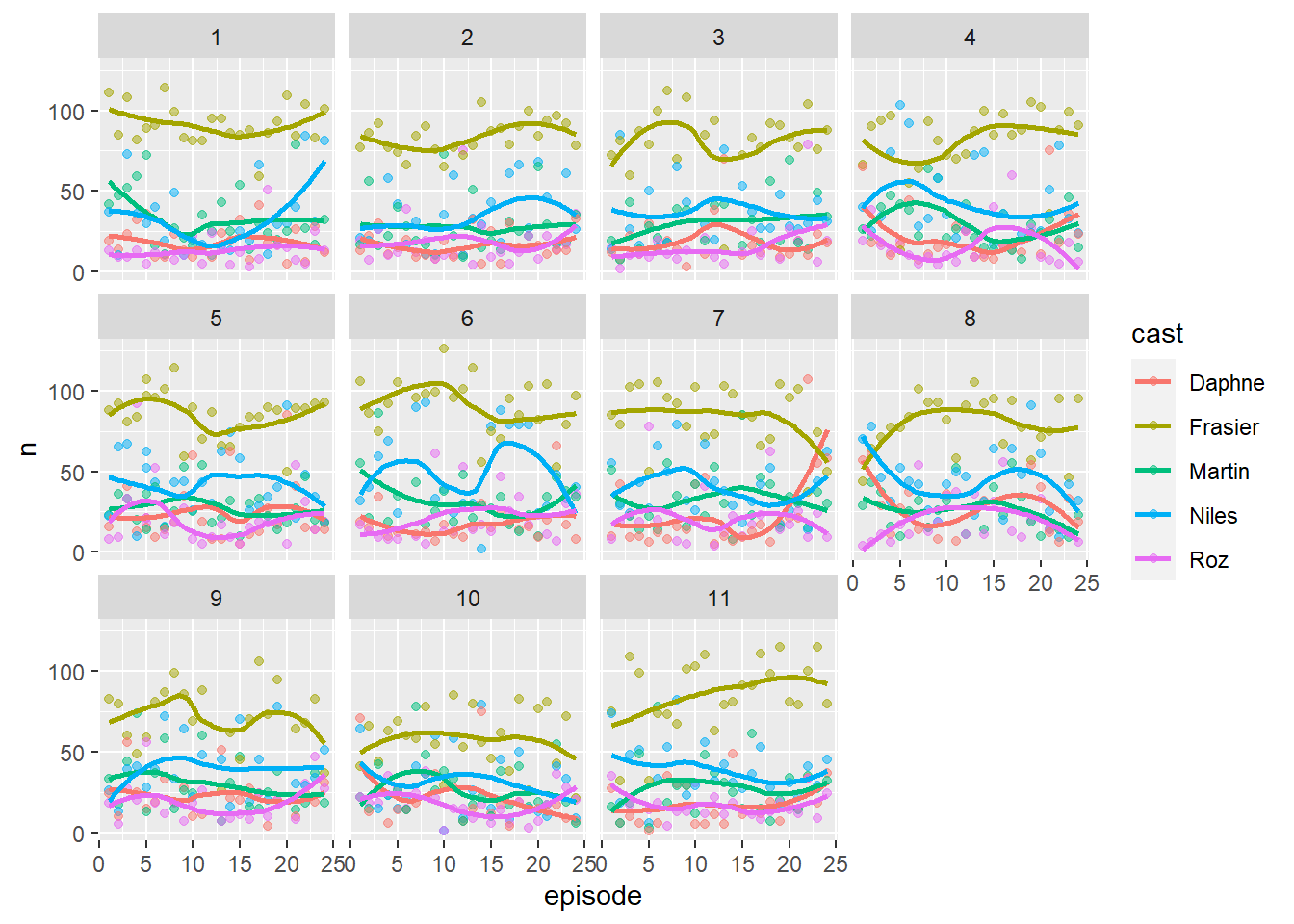
Frasier almost always gets 80-90 lines per episode for instance, but there are exceptions. The final episode of season 7 and the first episode of season 8 for instance see Daphne and Niles dominating, and fans of the show will realise that these are the two episodes where they got married.
I think it’s also interesting to note how all of the main characters like Martin or Roz have an episode or two where they get the 2nd highest number of lines. It’s a testament to how much the writers emphasised on character development.
Writers & Directors
Since we also have episode meta data, it would be interesting to see how different writers and directors contributed to the show.
By terms of sheer volumes, it would look something like this:
episode %>%
  group_by(writers) %>%
  count(sort = T) %>%
  head(20) %>%
  ggplot(aes(fct_reorder(writers, n), n, fill = writers)) +
  geom_col()+
  coord_flip()+
  xlab("Writers")+
  ylab("Number of Episodes")+
  labs(title = "20 Most Prolific Frasier Writers")+
  theme(legend.position = "none")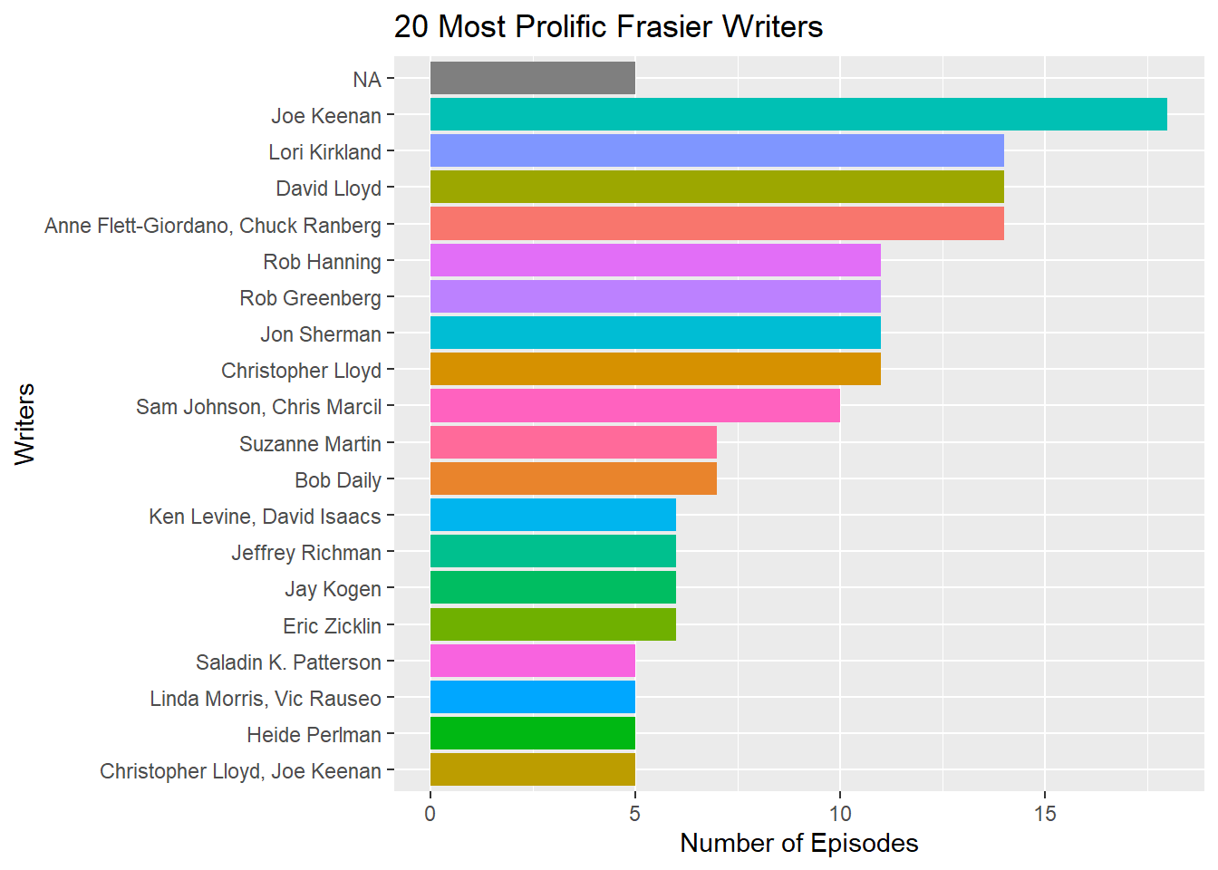
episode %>%
  group_by(directors) %>%
  count(sort = T) %>%
  head(20) %>%
  ggplot(aes(fct_reorder(directors, n), n, fill = directors)) +
  geom_col()+
  coord_flip()+
  xlab("Directors")+
  ylab("Number of Episodes")+
  labs(title = "20 Most Prolific Frasier Directors")+
  theme(legend.position = "none")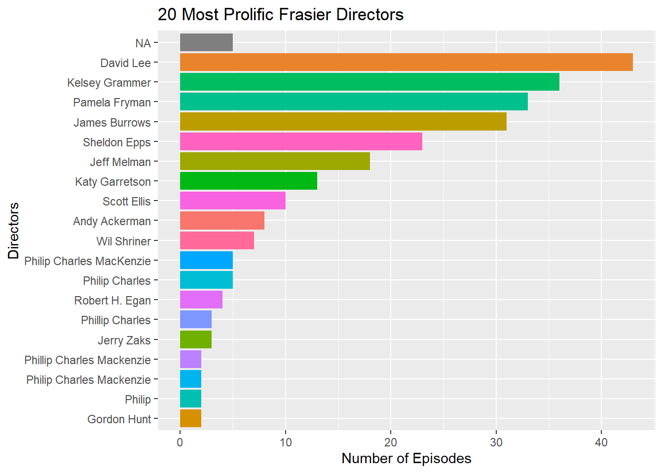
But we also have the IMDB ratings of the entire show:
ggplot(episode,(aes(imdb_rating)))+
  geom_histogram(bins = 20)
## Warning: Removed 6 rows containing non-finite values (stat_bin).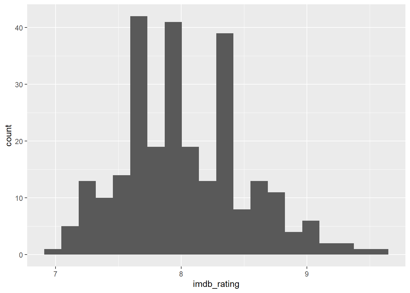
Which means we can be creative and see if any writers or directors contribute to a better IMDB rating. To do this, we’ll turn each director and writer into a column in our dataset, and dummy code with a 1 if he contributed to that episode.
There are many different ways of doing this, but in this case I’ll use the fastDummies package.
categorical_variables <- episode %>%
  select(url, writers, directors) %>%
  fastDummies::dummy_cols(select_columns = c("writers", "directors")) %>%
  distinct()
And just to give you an idea what that looks like, here are the first 5 rows of a tiny slice:
head(categorical_variables[4:6])## # A tibble: 6 x 3
## `writers_Alex Gregory, P~ `writers_Anne Flett-G~ `writers_Anne Flett-Giordano~
## <int> <int> <int>
## 1 0 0 0
## 2 0 0 0
## 3 0 0 1
## 4 0 0 0
## 5 0 0 0
## 6 0 0 0Since there are 34 different directors and 76 different writers, this means we’ve added 110 columns to our dataframe. And since the code for a few additional features (if an episode features Maris, Word count and sentiment) are already done, I’ve decided to appent these as well!
This part of the data also has our IMDB rating, which will be our predictor variable, and the episode url, which we’ll use to join the categorical and non-categorical data together.
noncategorical_variables <- episode %>%
  select(url, season, episode, imdb_rating) %>%
  left_join(WordsperEpisodeFE) %>%
  left_join(SentimentAnalysisFE) %>%
  left_join(MarisFE) %>%
  distinct()
## Joining, by = "url"
## Joining, by = "url"
## Joining, by = "url"head(noncategorical_variables)## # A tibble: 6 x 7
## url season episode imdb_rating WordsperEpisode episode_sentime~ CountMaris
## <chr> <dbl> <dbl> <dbl> <int> <dbl> <int>
## 1 http:/~ 1 1 8.6 3325 0.249 4
## 2 http:/~ 1 2 8.1 2916 0.328 0
## 3 http:/~ 1 3 8.2 3364 0.620 5
## 4 http:/~ 1 4 7.9 3252 0.386 2
## 5 http:/~ 1 5 8 3360 0.578 1
## 6 http:/~ 1 6 7.7 3263 0.440 3features <- categorical_variables %>%
left_join(noncategorical_variables) %>%
select(-c(url, writers, directors)) %>%
drop_na()## Joining, by = "url"After the join, I removed the url, since it’s simply a unique case ID, and the original writers and directors columns, which have now become redundant, because we’re capturing that information through our dummy variables.
Elastic Net Regression
Rather than create a model to predict IMDB ratings, what we want to do is see which features contribute most to that rating score. One powerful statistical method that does this feature selection and handles wide datasets well is elastic net.
Elastic nets are implemented in R through the glmnet library, but to use that, we’ll have to turn our dataframe into a matrix, and split the target and features into separate matrices, since glmnet does not accept the usual predictor ~ variables formula notation.
After that’s done, fitting a model is relatively straightforward. We’ll use the cv.glmnet function, which does 10 cross validation folds by default.
set.seed(31)
y <- matrix(features$imdb_rating)
X <- features %>% select(-imdb_rating) %>% data.matrix()

glmnet_model <- cv.glmnet(X, y, type.measure = "mse")
plot(glmnet_model)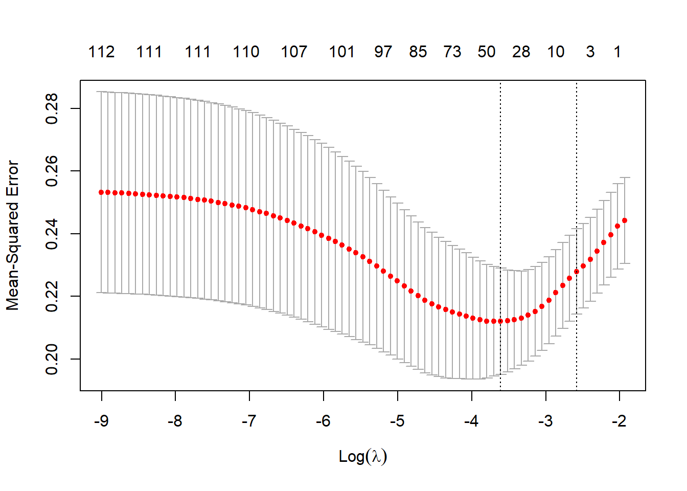
The plot shows us the MSE as glmnet iterates through different values of the regularization parameter lambda. Our mean squared error is between 0.22 and 0.26 IMDB points: which means we’re predicting IMDB ratings that are usually just a quarter of a point off.
Now comes the really fun part. We can see which features elasticnet decided to penalize because they were unimportant, and conversely, we can see which features were important, and their relative importance.
And we can graph that out into something like this:
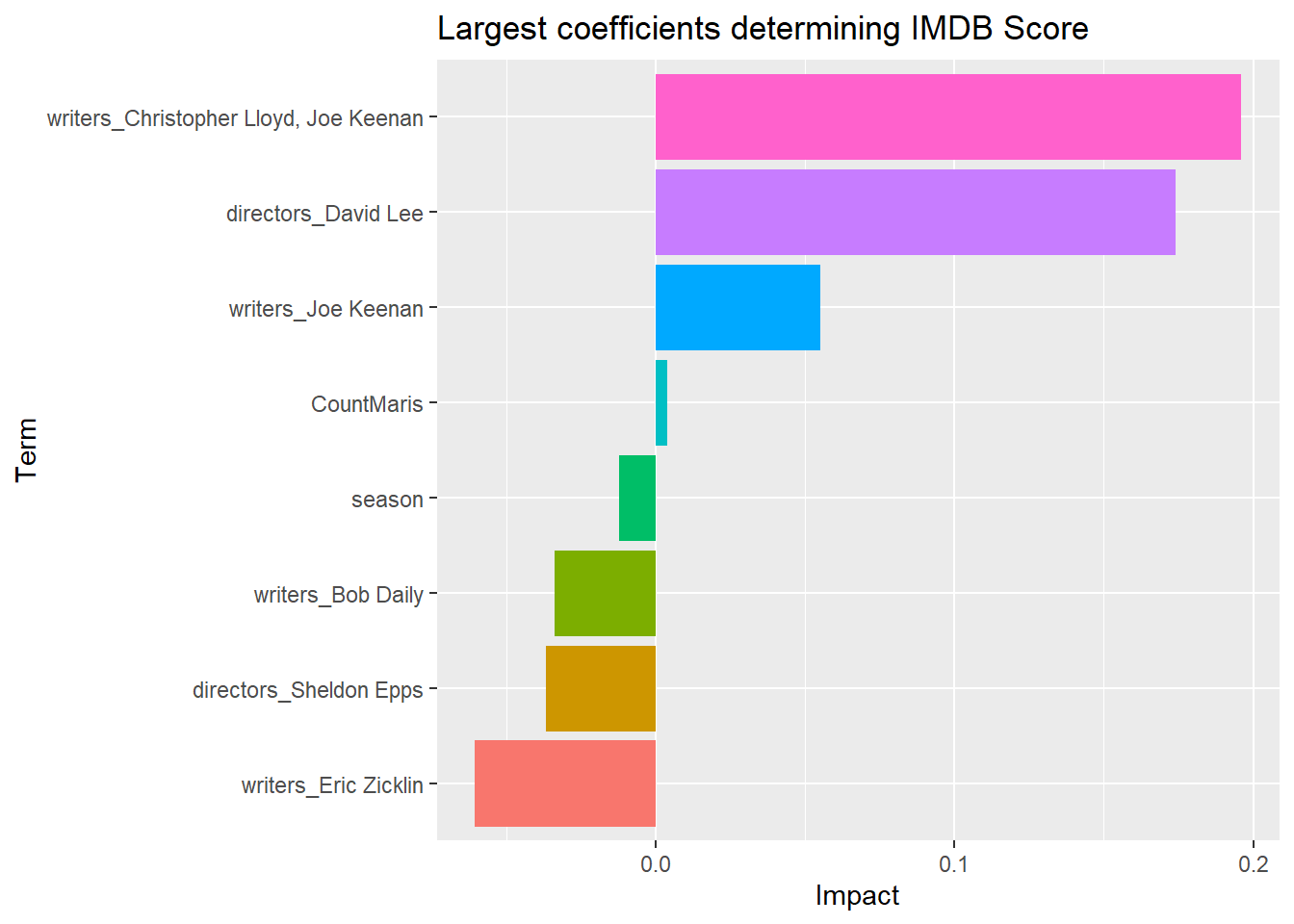
If the coeffecient, or what I named “impact” is positive, it means those variables increase the IMDB score. So episodes written by Christopher Lloyd or Joe Keenan or directed by David Lee tend to get a higher IMDB rating.
Episodes with higher counts of Maris also are higher rated, although this effect is slight. And, as season gets larger (and we get later into the show), the ratings dip a bit compared to the start. Which makes sense when you plot it!
ggplot(episode, aes(Aired_date, imdb_rating))+
  geom_point()+
  geom_smooth(method = "lm", se = F)
## `geom_smooth()` using formula 'y ~ x'## Warning: Removed 63 rows containing non-finite values (stat_smooth).## Warning: Removed 63 rows containing missing values (geom_point).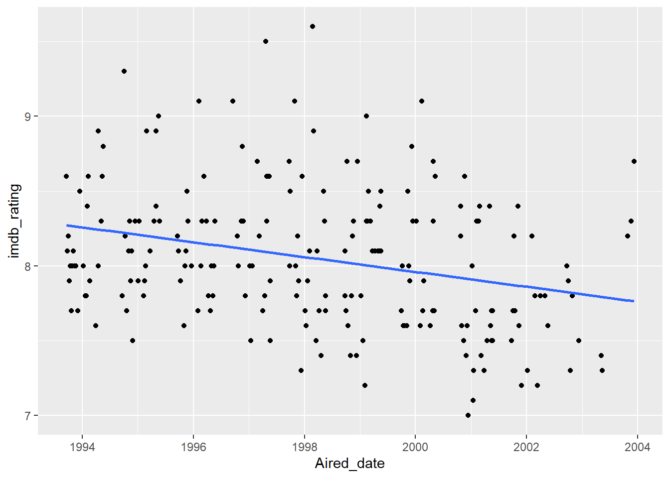
And it turns out that Joe Keenan did indeed write some of my favourite episodes of the entire show:
episode %>% filter(writers == "Joe Keenan") %>% select(season, episode, title)## # A tibble: 18 x 3
## season episode title
## <dbl> <dbl> <chr>
## 1 2 3 The Matchmaker
## 2 2 6 The Botched Language Of Cranes
## 3 2 15 You Scratch My Book...
## 4 2 22 Agents In America, Part Three
## 5 3 7 The Adventures of Bad Boy and Dirty Girl
## 6 3 15 A Word To The Wiseguy
## 7 3 21 Where There's Smoke There's Fired
## 8 4 1 The Two Mrs. Cranes
## 9 4 9 <NA>
## 10 4 17 Roz's Turn
## 11 5 12 The Zoo Story
## 12 5 14 The Ski Lodge
## 13 6 8 The Seal Who Came To Dinner
## 14 6 20 Dr. Nora
## 15 7 4 Everyone's A Critic
## 16 7 15 Out With Dad
## 17 11 3 The Doctor Is Out
## 18 11 15 Caught In The ActIt probably would be fitting to end a post about Frasier with a clip on some outtakes.
I really can’t emphasise enough how great of a show it is, so if you’ve never seen an episode, I’d encourage you to give it a try.