Intro
The Department of Maltese at the University of Malta launched a splendid website available here, and it also spotlights some of the dissertations by its students. Two of them immediately piqued my attention, Il-kelma Maltija ta’ Eddie Fenech Adami by James Aaron Ellul and L-arti tal-kelma fid-diskorsi politiċi ta’ Duminku Mintoff (1962) by Christabelle Borg.
Both dissertations included sizable appendices with political speeches that are relatively hard to come by on the web, so I got curious to see what some old school text mining can reveal.
Loading the Speeches
I did a copy and paste job on the respective speeches and saved them into individual .txt files, read them in separately, added some date and speaker metainfo and cleaned away text in brackets that had the listener’s reactions like (clapping) or (shouts).
library(tidytext)
library(tidyverse)
library(readr)
library(scales)
library(lubridate)


efa <- paste0("efa_", seq(1,4, by = 1), ".txt") %>%
  map(~read_file(paste0("~/RProjects/Historic Political Speeches/Input/", .x))) %>%
  unlist() %>%
  as.data.frame() %>%
  bind_cols(data.frame(speech = dmy(c("14 Dec 1986",
                                  "1 Feb 1987",
                                  "8 Mar 1987",
                                  "30 Jan 2003")))) %>%
  mutate(speaker = "Fenech Adami")

mintoff <- paste0("mintoff_", seq(1,7, by = 1), ".txt") %>%
  map(~read_file(paste0("~/RProjects/Historic Political Speeches/Input/", .x))) %>%
  unlist() %>%
  as.data.frame() %>%
  bind_cols(data.frame(speech = dmy(c("14 Jan 1962", "21 Jan 1962",
                                  "28 Jan 1962", "4 Feb 1962",
                                  "11 Mar 1962", "29 Apr 1962",
                                  "21 Oct 1962")))) %>%
  mutate(speaker = "Mintoff")

speeches <- efa %>%
  bind_rows(mintoff) %>%
  rename(text = ".") %>%
  mutate(text = str_replace(text, "\\([^()]+\\)", ""))
Creating Bag of Words Model
Our first step is to transform the speeches into a traditional bag of words model, where each word said by a speaker in a particular speech is counted. We end up with something like the below:
speeches_tidied_tokens <- speeches %>%
    unnest_tokens(word, text) %>%
  group_by(speech, speaker, word) %>%
  tally(sort=T) %>%
  ungroup()

head(speeches_tidied_tokens, 15)
## # A tibble: 15 x 4
## speech speaker word n
## <date> <chr> <chr> <int>
## 1 1987-03-08 Fenech Adami li 487
## 2 1986-12-14 Fenech Adami li 308
## 3 1987-02-01 Fenech Adami li 291
## 4 1987-03-08 Fenech Adami l 273
## 5 1987-03-08 Fenech Adami u 250
## 6 1962-01-14 Mintoff u 220
## 7 1962-01-21 Mintoff u 219
## 8 1962-10-21 Mintoff u 218
## 9 1987-03-08 Fenech Adami il 211
## 10 1986-12-14 Fenech Adami il 209
## 11 1962-02-04 Mintoff u 199
## 12 1962-03-11 Mintoff u 188
## 13 1986-12-14 Fenech Adami l 180
## 14 1962-03-11 Mintoff li 175
## 15 1962-03-11 Mintoff l 172Immediately, we notice that the most frequent words are the Maltese articles like “li”, “u” and “il”. These are considered to have next to no information, and are frequently filtered out by using a list of stopwords such as this. However, I couldn’t find one for Maltese, so we’ll have to get more creative.
Zipf’s Law
In the beginning of the 1900’s, a few smart people including the French stenographer Jean-Baptiste Estoup and the American Linguist George Kingsley Zipf began to notice that a consistent pattern emerged across different languages: a few words were used a great deal, while many were rarely used.
More specifically, the frequency of a word is often inversely proportional to it’s rank, with the second most common word occurring only half as frequently as the first, and the third only occurring a third as frequently as the first.
Put graphically, if we calculate the word frequency in our speeches, it would look like this:
word_freq <- speeches_tidied_tokens %>%
  select(-c(speaker, speech)) %>%
  group_by(word) %>%
  summarise(n = sum(n)) %>%
  arrange(desc(n)) %>%
  mutate(rank = row_number(),
         term_frequency = n/sum(n)) %>%
  ungroup()

word_freq %>%
ggplot(aes(rank, term_frequency)) +
  geom_line(col = "blue") +
  theme_bw()+
  ylab("Frequency of Word")+
  xlab("Word Rank")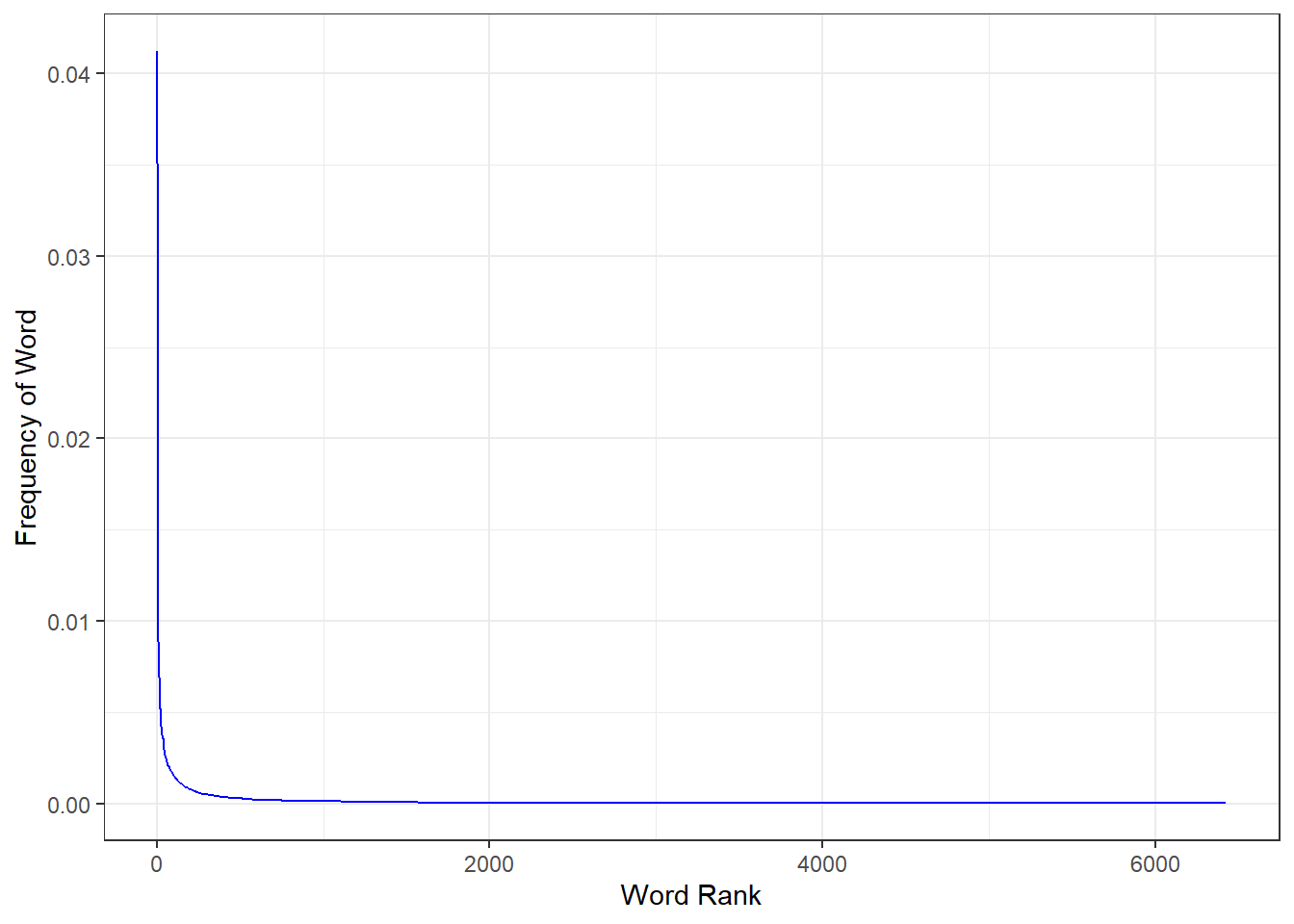
This behavior isn’t just limited to languages, and is found in many other domains, especially human constructed ones. The wikipedia article on Zipf’s Law goes into more detail.
It’s the custom to plot power laws on a log-log scale like this to make the relationship more clear:
word_freq %>%
  filter(n>2) %>%
ggplot(aes(rank, term_frequency, label = word)) +
  geom_line(col = "blue") +
  scale_y_log10(labels = comma)+
  scale_x_log10()+
  theme_bw()+
  geom_text(check_overlap = T, nudge_y = .2)+
  ylab("Frequency of Word")+
  xlab("Word Rank")+
  labs(title = "Zipf's Law in Maltese Political Speeches")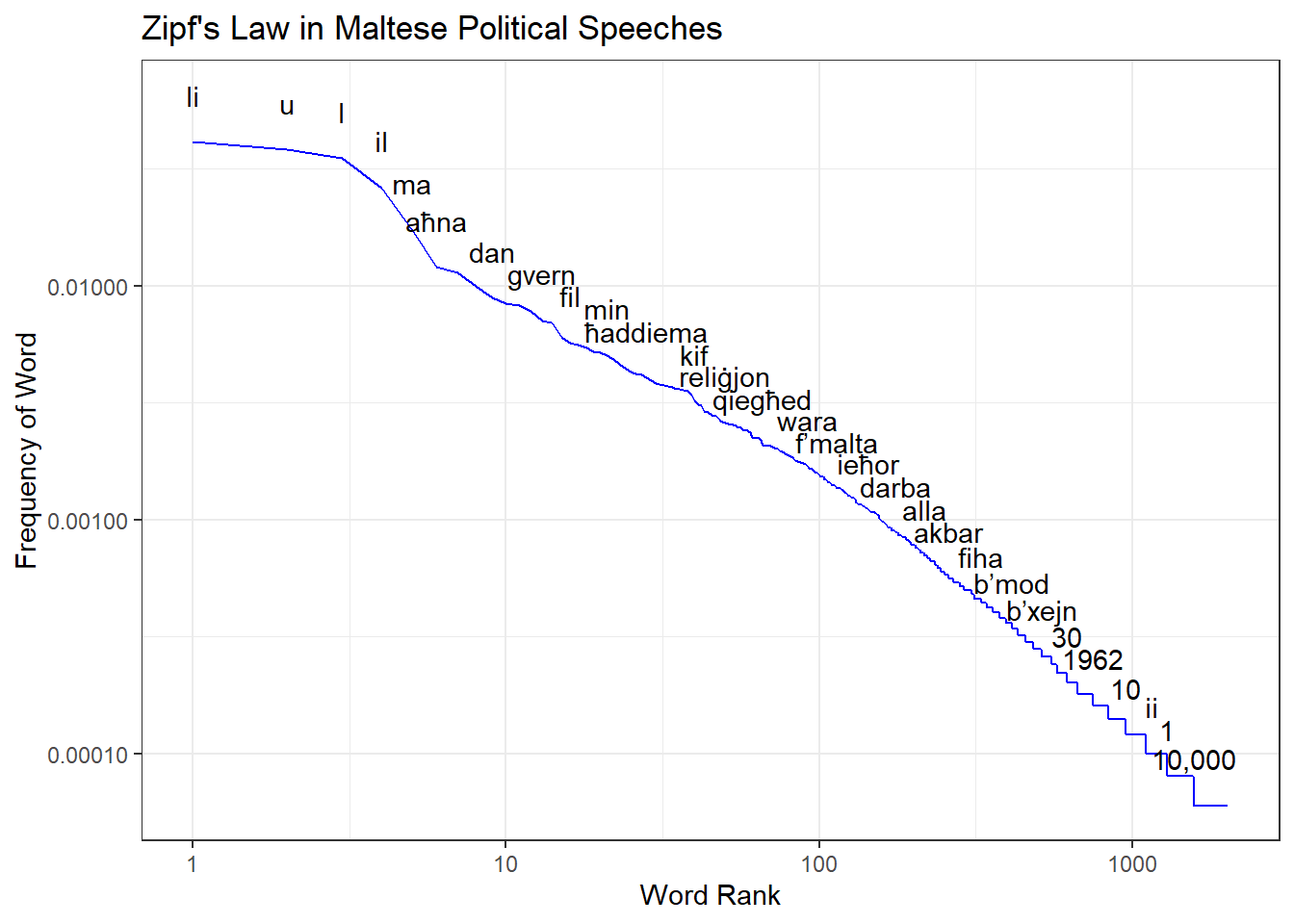
Get Stopwords List
So using what we know about Zipf’s law, we can create a custom Maltese stoplist by taking, say, the top 70 words by frequency:
word_freq_stopwords <-
  word_freq %>%
  select(word) %>%
  head(70)
And to see how well it works, we can quickly plot the top 40 words
speeches_tidied_tokens %>%
  group_by(speaker, word) %>%
  summarise(n = sum(n)) %>%
  anti_join(word_freq_stopwords) %>%
  arrange(desc(n)) %>%
  head(40) %>%
  ggplot(aes(fct_reorder(word, n), n, fill = speaker))+
  geom_col()+
  coord_flip()+
  facet_wrap(~speaker)+
  theme_bw()+
  ylab("Word")+
  xlab("Frequency")+
  theme(legend.position = "none")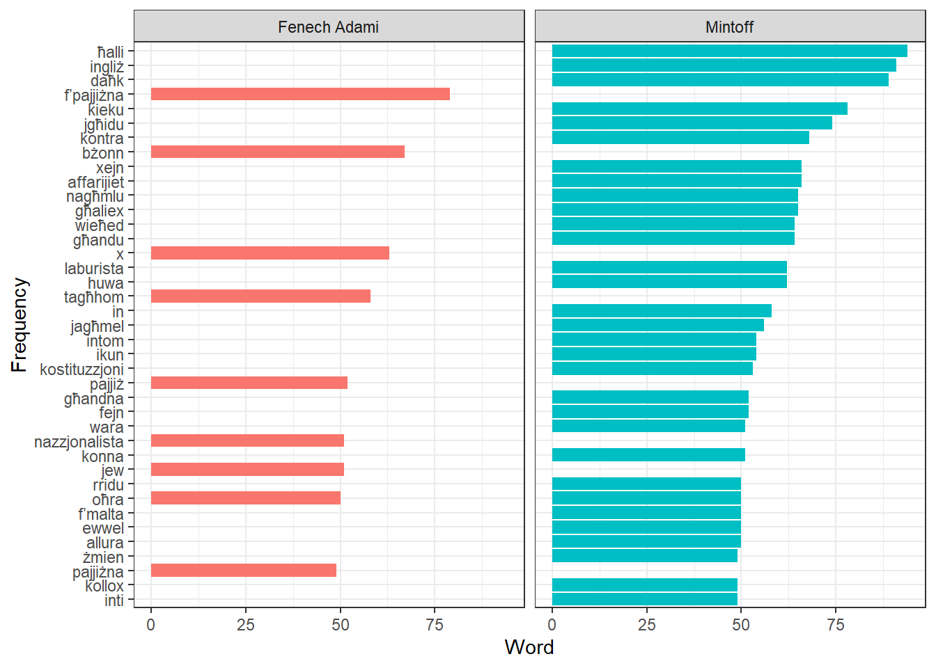
Seems like we’re getting somewhere! But we can do more to sift the signal from the noise!
TF-IDF
Term frequency–inverse document frequency is a statistic that measures how prevalent a word is for a particular document in a set of documents. In our case, “documents” are speeches, and if all 11 speeches mentioned the word “government” the same number of times, this term would have a high term frequency but low inverse document frequency. But if the word “union” appears many times in just one speech, it would have just what we want: a term frequency weighted upward by a relatively high idf.
Much of the theory behind tf-idf is now well over half a century old, and it’s very much seen as several decades past the cutting edge in favour of fancier approaches, but the gist of tf-idf probably lives on in highly optimized search ranking functions all over the web.
So what do you get when you feed the speeches into a tf-idf algorithm? Here’s the result, sorted by chronological order of the speech.
tf_idf <- speeches_tidied_tokens %>%
  bind_tf_idf(word, speech, n)

tf_idf %>%
  group_by(speech) %>%
  slice_max(tf_idf, n = 6) %>%
  ungroup() %>%
  ggplot(aes(tf_idf, fct_reorder(word, tf_idf), fill = speaker)) +
  geom_col() +
  facet_wrap(~speech, ncol = 3, scales = "free") +
  labs(x = "tf-idf", y = NULL)+
  scale_fill_manual(values = c("#00BFC4", "#F8766D"))+
  theme(legend.position="bottom")+
  labs(title = "Top tf-idf terms by speech")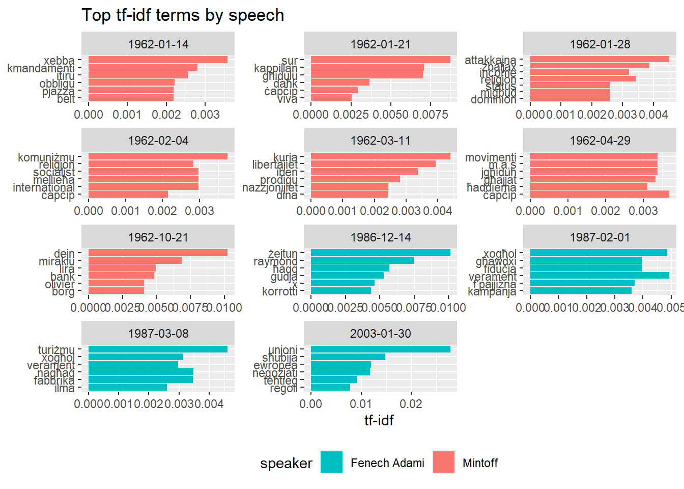
The results are actually quite fun. On Mintoff’s speech on the 14th of January, “xebba”, “kmandamenti” and “itiru” stand out as noteworthy. If you’re wondering what he did with that, his speech was against the Catholic Church’s interdiction of his party that had just happened the previous year. The “xebba” was Joan or Arc, who Mintoff said was burned at the stake because she stepped on the toes of some bishops.
The other two are too hilarious not to reproduce here.
3,000 sena ilu, Mosè niżel mill-muntanja b’żewġ tabelli tal-irħam, u qal lill-poplu Lhudi: Dawn huma l-kmandamenti t’Alla. U kienu 10 kmandamenti t’Alla. U ilhom dawn il-kmandamenti 3,000 sena, u l-insara kollha tad-dinja jqimuhom dawn u jibqgħu jqimuhom dawn l-10 kmandamenti t’Alla. X’għamlu n-nies ta’ żminijietna? Ma’ dawn l-għaxar kmandamenti llum, żiedu l-ħdax u qalu: min jaqra l-Ħelsien jagħmel dnub. Żiedu t-tnax u qalu: min ibigħ il-Ħelsien jagħmel dnub mejjet. Żiedu t-tlettax u qalu: min iqassam il-Ħelsien jagħmel dnub mejjet, bit-2/6. Żiedu l-erbatax: min imur il-meetings Laburisti jagħmel dnub mejjet. U minn issa sakemm tiġi l-elezzjoni min jaf kemm għad iridu jżidu l-kmandamenti. U aħna ngħidulu lil dawn: U dana mhux Mosè żiedhom dawn il-kmandamenti minn fuq il-muntanja bl-ordni t’Alla, dawn waħħluhom xi erba’ qtates kontra tagħna, dawn il-kmandamenti.
Aħna, il-Maltin, ilkoll niftakru x’għamlulu lil Strickland. Kemm qalu fi żmien Strickland u l-Laburisti, itiru, itiru, qalu bil-ġwienaħ itiru. Jindilku, intom tidħqu qegħdin illum, imma dakinhar, in-nies ta’ dakinhar, tgħidx x’kien hawn, kemm kien hawn min belagħha. Meta Strickland u l-Laburisti għandhom l-ingwent, jindilku, u kif jidilku l-ingwent itiru, itiru. Idħqu, idħqu illum. Ma tafux dakinhar. Min jaf kemm kien hawn min isodd it-toqob tal-ventilaturi dakinhar biex ma jidħlux ta’ Strickland billejl.
The two speeches later in January continue on the religious issue, but we also see “dominion” pop up, in reference to Mintoff’s foreign policy plan of attempting to integrate Malta within the broader UK as a “dominion”. The sole speech in February mostly concerns the visit to Communist International congress, while March’s speech is a reply to a pastoral letter by the archbishop inviting Labour supporters back into the Church as “prodigal sons”, which as you can imagine was received swimmingly.
The final Mintoff speech is about internal fiscal policy, where he accuses the Borg Olivier government of driving the nation several thousands of “liri” into debt.
Fenech Adami’s first speech is a few days after the murder of Raymond Caruana, so those events are discussed, together with a pledge against corruption and for justice.
His second speech was in Gozo, and “Ghawdxi” peaks. “Kampanja” is a reference to the electoral campaign, which Fenech Adami said was in full swing, to deliver a government that would create equal opportunities for work for all.
We also see a quirk developing in Fenech Adami’s second and third speeches: his fondness for the word “verament”.
The “fabrika” term also seems to have a humorous story:
tiftakru fabbrika oħra kbira li fetħet u għalqet fi żmienhom stess, fabbrika Ġappuniża, li kienet timpjega mijiet ta’ ħaddiema Maltin. Din kienet fabbrika b’teknoloġija moderna li riedet tbiddel il-prodott li kienet tipproduċi. Niftakar li wħud milli kienu responsabbli għaliha kienu ġew kellmuni qabel m’għalqet u qaluli li huma kienu lesti li jkomplu jaħdmu f’Malta. Riedu biss li jkunu jistgħu jipproduċu televisions tal-kulur. Imma Mintoff li jaf kollox, Mintoff li ma kien imerih ħadd, għax dawk l-Ministri kollha li issa jgħidu kontra tiegħu ma kienux jazzardaw imeruh f’xi ħaġa, Mintoff fis-sapjenza kbira tiegħu kien qal l-poplu Malti m’għandux jixtri televisions tal-kulur.
U biex il-Maltin ma jixtrux televisions tal-kulur, lil dawn ma tagħhomx permess li jagħmlu t-televisions tal-kulur u l-fabbrika għalqet u mijiet ta’ ħaddiema Maltin tilfu l-post tax-xogħol tagħhom.
The final speech is on the day after Fenech Adami set the date for the EU membership referendum.
Not a bad signal to noise ratio for such an old algorithm, right?
Word Frequency Scatter Plot
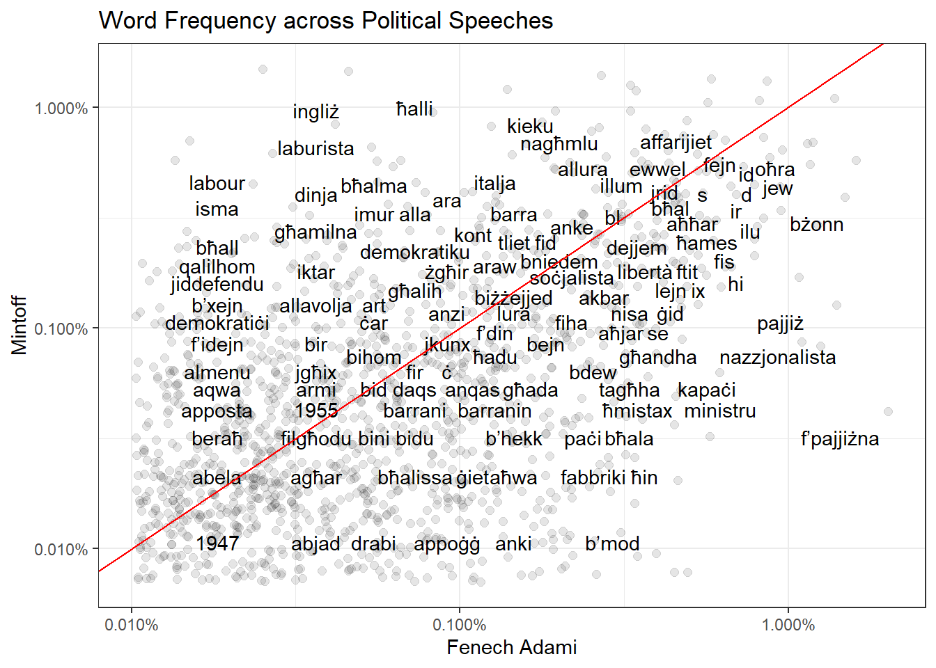
Another thing we can do is plot words by frequency, with Mintoff on one axis and Fenech Adami on another. You’re equally likely to hear words along the red 45 degree diagonal in both mass meetings, with words at the top right of the graph being the most popular.
Words clustered in the top left area are generally unique to Mintoff mass meetings, while words clustered on the bottom right are unique to Fenech Adami mass meetings.
1947 and 1955 seem to be references to those respective general elections.
Speech Length
Fenech Adami’s speeches are also much more variable in length - he has both the longest (8,351) and shortest (1,837) speeches in the corpus. Mintoff’s are consistently around the 4,000 word mark.
speeches_tidied_tokens %>%
  group_by(speech, speaker) %>%
  summarise(sum(n)) %>%
  ungroup() %>%
  ggplot(aes(x = speaker, y = `sum(n)`, fill = speaker))+
  geom_violin()+
  theme_bw()+
  ylab("Words")+
  xlab("")
## `summarise()` has grouped output by 'speech'. You can override using the `.groups` argument.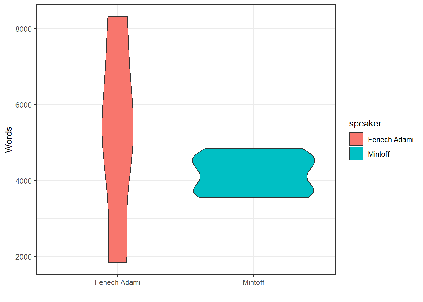
Topic Modeling
Perhaps the most powerful variation of bag of word approaches is topic modeling. Topic modeling launches from the rather basic assumption that documents are a collection or words. “Topics” are also represented by different collections of words, and every document can have a mixture of these topics.
For instance, taking our corpus as an example, we might have a topic that contains “EU”, “membership”, “Euro” and “negotiation”, which we label as “EU Affairs”. Our speeches will reflect a proportion of this topic (if the speech was entirely about joining the Eurozone, it will be high, maybe 80% or even 100%, while if the speech was about Joan or Arc, it might even be 0%).
One of the most popular topic modeling algorithms is Latent Dirichlet Allocation and many “speed reading” services employ it to distill what a vast collection of text is about.
If you’re curious about how LDA works, this is a very friendly introduction by Luis Serrano.
But in short, an LDA algorithm takes our words in the form of a matrix as an input, and the number of clusters or “topics” we want it to find - in my case I opted for 9 for the simple reason that it fits nicely into a 3x3 graph.
library(topicmodels)

lda <- speeches_tidied_tokens %>%
  anti_join(word_freq_stopwords) %>%
  cast_dtm(document = speech, word, n) %>%
  LDA(k = 9, control = list(seed = 19032021))

topics <- tidy(lda, matrix = "beta")

top_terms <- topics %>%
  group_by(topic) %>%
  top_n(10, beta) %>%
  ungroup() %>%
  arrange(topic, -beta)

top_terms %>%
  mutate(term = reorder_within(term, beta, topic)) %>%
  ggplot(aes(beta, term, fill = factor(topic))) +
  geom_col(show.legend = FALSE) +
  facet_wrap(~ topic, scales = "free") +
  scale_y_reordered()+
  labs(title = "Inferred Topic")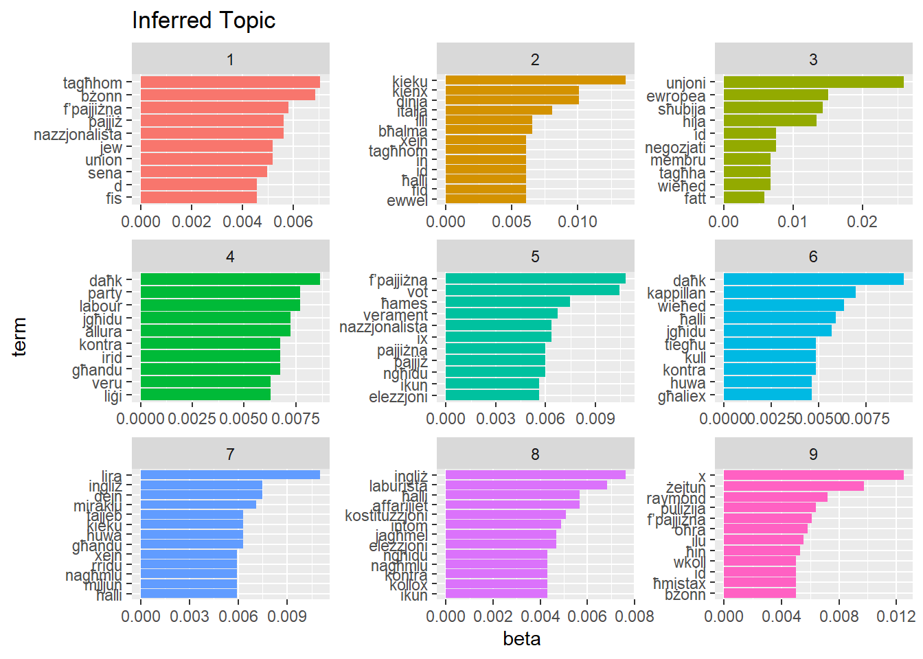
With that, we can then rename the clusters with what we infer from them:
topic_labels <- tibble(topic = c(1:9),
                       label = c("PN Pledges",
                       "",
                       "EU",
                       "Religious Issues",
                       "PN Pledges",
                       "Religious Issues",
                       "Gvmt. Debt",
                       "UK Relations",
                       "Raymond Caruana"))

topic_labels
## # A tibble: 9 x 2
## topic label
## <int> <chr>
## 1 1 "PN Pledges"
## 2 2 ""
## 3 3 "EU"
## 4 4 "Religious Issues"
## 5 5 "PN Pledges"
## 6 6 "Religious Issues"
## 7 7 "Gvmt. Debt"
## 8 8 "UK Relations"
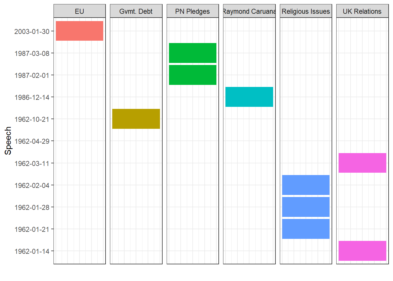
## 9 9 "Raymond Caruana"Then, we can plot which speeches discussed which topics:
gamma <- tidy(lda, matrix = "gamma") %>%
  mutate(document = ymd(document)) %>%
  inner_join(topic_labels)

gamma %>%
  filter(topic != 2) %>%
  ggplot(aes(factor(document), gamma, fill = label)) +
  geom_col() +
  coord_flip()+
  facet_wrap(~ label, ncol = 6) +
  labs(x = "Speech", y = "")+
  theme_bw()+
  theme(legend.position = "none")+
  theme(axis.text.x=element_blank(),
        axis.ticks.x=element_blank())